Sigmoid functions are a type of mathematical function that has a characteristic “S” shape. They are commonly used in mathematical modeling to represent a variety of phenomena, such as the probability of an event occurring, the growth of a population, or the spread of a disease. They naturally exhibit the property of gradual then sudden increase without exploding. I use sigmoids all the time for fitting data. They are smooth and differentiable, as well as being easy to add boundary conditions to. In this post, I provide some tips for how to adapt them to different problem cases.
from typing import Callable

import numpy as np
from matplotlib import pyplot as plt
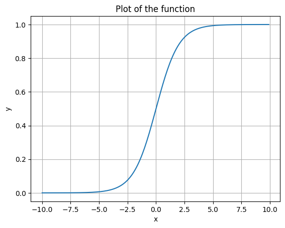
Here’s the basic sigmoid function:
def sigmoid(x: float) -> float:
    """
    Compute the sigmoid function for the input value x.
    For any output between negative infinity and positive infinity, it returns a response between 0 and 1
    """
    return 1 / (1 + np.exp(-x))
Let’s see what it does.
print(sigmoid(1))
print(sigmoid(0))
print(sigmoid(10))
print(sigmoid(-99))
0.7310585786300049
0.5
0.9999546021312976
1.0112214926104486e-43
Now let’s make a function to plot functions so we can visualize them.
def plot_function(func: Callable, start: float = -10, end: float = 10, step: float = 0.1, **kwargs):
    """
    Plot the given function within the specified range and step.

    Args:
        func: A function to plot.
        start: Start value of the x-axis range.
        end: End value of the x-axis range.
        step: Step size for x-axis values. Default is 0.1.
    """
    x_values = np.arange(start, end, step)
    y_values = func(x_values, **kwargs)

    plt.plot(x_values, y_values)
    plt.xlabel("x")
    plt.ylabel("y")
    plt.title("Plot of the function")
    plt.grid(True)
    plt.show()
plot_function(sigmoid)

Let’s say we want to use to it model something. The y-bounds at 0 and 1 aren’t necessarily what we want. Nor is the inflection point at x=0 or the amount of stretch. To allow us to tweak these, let’s write a new sigmoid function that gives us parameters to play with.
def sigmoid(x, x_shift=0, y_shift=0, x_scale=1, y_scale=1):
    """
    Parameterized sigmoid function
    """
    x_transformed = (x - x_shift) / x_scale
    sigmoid_value = 1 / (1 + np.exp(-x_transformed))
    y_transformed = y_scale * sigmoid_value + y_shift
    return y_transformed
We can see that the base case is the same.
plot_function(sigmoid)
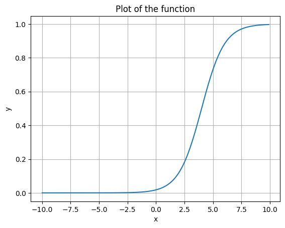
But now we can also move it around. Let’s slide it to the right.
plot_function(sigmoid, x_shift=4)
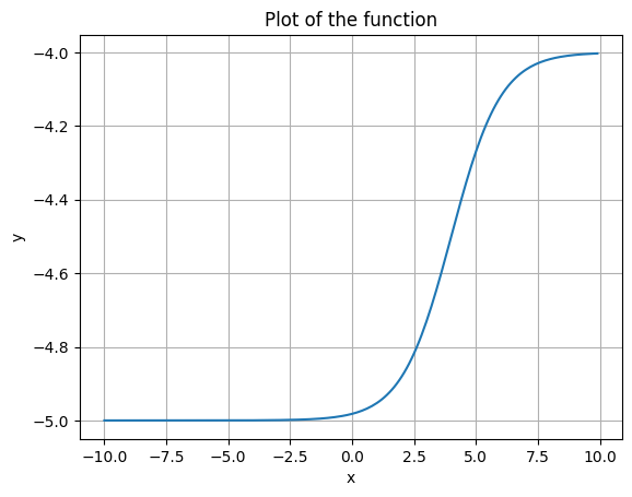
Now drop it down.
plot_function(sigmoid, x_shift=4, y_shift=-5)
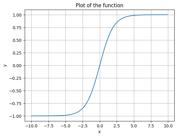
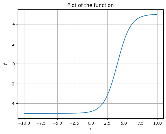
Now stretch it in the y-axis. Note the change in the y-axis labels below.
plot_function(sigmoid, x_shift=4, y_shift=-5, y_scale=10)
Depending on your use case, you may want to specify certain conditions. For example, say you wanted to specify the min and max of the function. There’s no explicit parameter for that, so we’ll have to figure out how to express that given the parameters we have. The two that we care about for this case are y_shift and y_scale. The x_shift and x_scale parameters could be anything in this case because we haven’t specified them. We could add additional constraints for them, but in this example, I’ll simply leave them alone. That leaves us with two unknowns, y_shift and y_scale, and two conditions, which we can solve for.
We know two points:
- x approaches infinity and y approaches the desired max
- x approaches negative infinity and y approaches the desired min
We’ll use \(\sigma\) to represent the sigmoid function.
Our starting formula is what we wrote in the sigmoid function:
\[\sigma(x) = \frac{y_\text{scale}}{1 + e^{-x_\text{scale}(x - x_\text{shift})}} + y_\text{shift}\]Now let’s plug in the following:
\[x = \infty\] \[y = max_\text{desired}\]Here’s what we get:
\[\sigma(\infty) = \frac{y_\text{scale}}{1 + e^{-\infty}} + y_\text{shift} = \frac{y_\text{scale}}{1 + 0} + y_\text{shift} = y_\text{scale} + y_\text{shift}\]Therefore:
\[y_\text{scale} + y_\text{shift} = max_\text{desired}\]At negative infinity, we’ve got:
\[\sigma(-\infty) = \frac{y_\text{scale}}{1 + e^{\infty}} + y_\text{shift} = \frac{y_\text{scale}}{\infty} + y_\text{shift} = y_\text{shift}\]Therefore:
\[y_\text{shift} = min_\text{desired}\]plugging this into the above equation, we have:
\[y_\text{scale} + min_\text{desired} = max_\text{desired}\]Ending with:
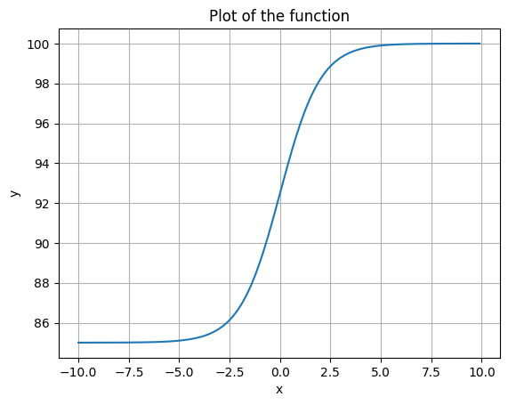
\[y_\text{shift} = min_\text{desired}\] \[y_\text{scale} = max_\text{desired} - min_\text{desired}\]Let’s give it a try.
desired_max = 100
desired_min = 85
y_shift = desired_min
y_scale = desired_max - desired_min
plot_function(sigmoid, y_shift=y_shift, y_scale=y_scale)
Another thing you might do is fit an equation with an inflection point and a desired max. Again, we have two equations and two unknowns.
Let’s start with our sigmoid equation again.
\[\sigma(x) = \frac{y_\text{scale}}{1 + e^{-x_\text{scale}(x - x_\text{shift})}} + y_\text{shift}\]We’ll start with the following:
\[x = \infty\] \[y = max_\text{desired}\]We already know the answer:
\[y_\text{scale} + y_\text{shift} = max_\text{desired}\]And therefore:
\[y_\text{shift} = max_\text{desired} - y_\text{scale}\]At the inflection point, we know that the inflection point in x is just x_shift, so we can say that \(x=x_\text{inflection}=x_\text{shift}\) and \(y = y_\text{inflection}\) (our desired point). Plugging that in, we get:
Plugging in \(y_\text{shift} = max_\text{desired} - y_\text{scale}\), we get:
\[\frac{y_\text{scale}}{2} + max_\text{desired} - y_\text{scale} = y_\text{inflection}\]Ending with:
\(y_\text{scale} = 2 * (max_\text{desired} - y_\text{inflection})\) \(y_\text{shift} = max_\text{desired} - y_\text{scale}\)
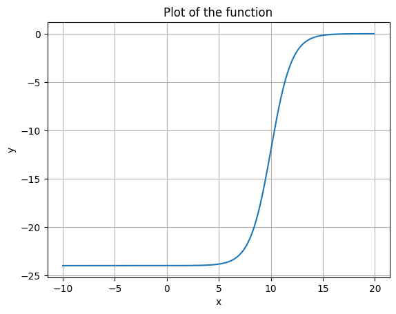
\[y_\text{scale} = 2 * (max_\text{desired} - y_\text{inflection})\] \[y_\text{shift} = max_\text{desired} - y_\text{scale}\]x_inflection = 10
y_inflection = -12
desired_max = 0
x_shift = x_inflection
y_scale = 2 * (desired_max - y_inflection)
y_shift = desired_max - y_scale
plot_function(sigmoid, -10, 20, x_shift=x_shift, y_shift=y_shift, y_scale=y_scale)
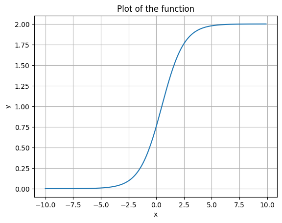
Let’s do another.
x_inflection = 0.5
y_inflection = 1
desired_max = 2
x_shift = x_inflection
y_scale = 2 * (desired_max - y_inflection)
y_shift = desired_max - y_scale
plot_function(sigmoid, x_shift=x_shift, y_shift=y_shift, y_scale=y_scale)
Last one:
x_inflection = 0
y_inflection = 0
desired_max = 1
x_shift = x_inflection
y_scale = 2 * (desired_max - y_inflection)
y_shift = desired_max - y_scale
plot_function(sigmoid, x_shift=x_shift, y_shift=y_shift, y_scale=y_scale)