
This post walks through recent work on Discovering Latent Knowledge in Language Models Without Supervision by Burns et al. The paper uses latent knowledge in the model’s activations to train the model. Their method answers yes-no questions accurately by identifying a direction in the activation space that adheres to logical consistency properties, such as having opposite truth values for a statement and its negation.
This post walks through the code to demonstrate the result. Much of it was taken directly from the author’s repo.
Table of Contents
import copy
import os

import matplotlib.pyplot as plt
import numpy as np
import pandas as pd
import plotly.express as px
import torch
import torch.nn as nn
import umap
from datasets import load_dataset
from matplotlib import pyplot as plt
from sklearn.decomposition import PCA
from sklearn.linear_model import LogisticRegression
from sklearn.manifold import TSNE
from sklearn.model_selection import train_test_split
from torchinfo import summary
from tqdm import tqdm
from transformers import AutoModelForMaskedLM, AutoTokenizer
np.random.seed(42)
Data
The authors tested their approach on various datasets and found that it worked. In this post, we’ll use the amazon polarity dataset for simplicity.
data = load_dataset("amazon_polarity")["test"]
Found cached dataset amazon_polarity (/home/julius/.cache/huggingface/datasets/amazon_polarity/amazon_polarity/3.0.0/a27b32b7e7b88eb274a8fa8ba0f654f1fe998a87c22547557317793b5d2772dc)


  0%|          | 0/2 [00:00<?, ?it/s]
Let’s take a look at the dataset.
for i in range(5):
    print(data[i])
    print()
{'label': 1, 'title': 'Great CD', 'content': 'My lovely Pat has one of the GREAT voices of her generation. I have listened to this CD for YEARS and I still LOVE IT. When I\'m in a good mood it makes me feel better. A bad mood just evaporates like sugar in the rain. This CD just oozes LIFE. Vocals are jusat STUUNNING and lyrics just kill. One of life\'s hidden gems. This is a desert isle CD in my book. Why she never made it big is just beyond me. Everytime I play this, no matter black, white, young, old, male, female EVERYBODY says one thing "Who was that singing ?"'}

{'label': 1, 'title': "One of the best game music soundtracks - for a game I didn't really play", 'content': "Despite the fact that I have only played a small portion of the game, the music I heard (plus the connection to Chrono Trigger which was great as well) led me to purchase the soundtrack, and it remains one of my favorite albums. There is an incredible mix of fun, epic, and emotional songs. Those sad and beautiful tracks I especially like, as there's not too many of those kinds of songs in my other video game soundtracks. I must admit that one of the songs (Life-A Distant Promise) has brought tears to my eyes on many occasions.My one complaint about this soundtrack is that they use guitar fretting effects in many of the songs, which I find distracting. But even if those weren't included I would still consider the collection worth it."}

{'label': 0, 'title': 'Batteries died within a year ...', 'content': 'I bought this charger in Jul 2003 and it worked OK for a while. The design is nice and convenient. However, after about a year, the batteries would not hold a charge. Might as well just get alkaline disposables, or look elsewhere for a charger that comes with batteries that have better staying power.'}

{'label': 1, 'title': 'works fine, but Maha Energy is better', 'content': "Check out Maha Energy's website. Their Powerex MH-C204F charger works in 100 minutes for rapid charge, with option for slower charge (better for batteries). And they have 2200 mAh batteries."}

{'label': 1, 'title': 'Great for the non-audiophile', 'content': "Reviewed quite a bit of the combo players and was hesitant due to unfavorable reviews and size of machines. I am weaning off my VHS collection, but don't want to replace them with DVD's. This unit is well built, easy to setup and resolution and special effects (no progressive scan for HDTV owners) suitable for many people looking for a versatile product.Cons- No universal remote."}
The labels correspond to the sentiment of the review. 1 indicates a positive review and 0 indicates a negative review.
Now let’s take a closer look at the text.
text = data[0]["content"]
text
'My lovely Pat has one of the GREAT voices of her generation. I have listened to this CD for YEARS and I still LOVE IT. When I\'m in a good mood it makes me feel better. A bad mood just evaporates like sugar in the rain. This CD just oozes LIFE. Vocals are jusat STUUNNING and lyrics just kill. One of life\'s hidden gems. This is a desert isle CD in my book. Why she never made it big is just beyond me. Everytime I play this, no matter black, white, young, old, male, female EVERYBODY says one thing "Who was that singing ?"'
Before it goes into the model we’ll need to convert the text into statements that are either true or false. To do that, we can create a new statement saying that the review is positive, and another to say that it’s negative. That way we’ll be guaranteed to have one true and one false statement.
def create_prompt_review(text: str, label: int) -> str:
    """
    Given a review (text) and its corresponding sentiment label (0 for negative or 1 for positive),
    creates a zero-shot prompt for the review by including the sentiment label as the answer.
    """
    sentiment = ["negative", "positive"][label]
    prompt = f"The following review expresses a {sentiment} sentiment:\n{text}"
    return prompt
create_prompt_review(text, 0)
'The following review expresses a negative sentiment:\nMy lovely Pat has one of the GREAT voices of her generation. I have listened to this CD for YEARS and I still LOVE IT. When I\'m in a good mood it makes me feel better. A bad mood just evaporates like sugar in the rain. This CD just oozes LIFE. Vocals are jusat STUUNNING and lyrics just kill. One of life\'s hidden gems. This is a desert isle CD in my book. Why she never made it big is just beyond me. Everytime I play this, no matter black, white, young, old, male, female EVERYBODY says one thing "Who was that singing ?"'
create_prompt_review(text, 1)
'The following review expresses a positive sentiment:\nMy lovely Pat has one of the GREAT voices of her generation. I have listened to this CD for YEARS and I still LOVE IT. When I\'m in a good mood it makes me feel better. A bad mood just evaporates like sugar in the rain. This CD just oozes LIFE. Vocals are jusat STUUNNING and lyrics just kill. One of life\'s hidden gems. This is a desert isle CD in my book. Why she never made it big is just beyond me. Everytime I play this, no matter black, white, young, old, male, female EVERYBODY says one thing "Who was that singing ?"'
Now we have statements that are either true or false. Let’s get the hidden states from them.
Extract hidden states
To do this, we’ll need to tokenize the text. Then we’ll run it through a model.
We’ll need to grab a tokenizer that’s right for our model. Fortunately, this is easy to do with AutoTokenizer.
# specify where to cache the model weights
cache_dir = os.getenv('MODELS')

# Set the model to the desired device (e.g., CPU or GPU)
device = torch.device("cuda" if torch.cuda.is_available() else "cpu")
We’ll use the deberta-v2-xxlarge model, so here we’ll grab the associated tokenizer.
model_type = "encoder"
tokenizer = AutoTokenizer.from_pretrained("microsoft/deberta-v2-xxlarge", cache_dir=cache_dir)
Special tokens have been added in the vocabulary, make sure the associated word embeddings are fine-tuned or trained.
Special tokens have been added in the vocabulary, make sure the associated word embeddings are fine-tuned or trained.
Let’s take a look at some of the attributes of the tokenizer.
print(f"Tokenizer Type: {type(tokenizer)}")
print(f"Model Type: {tokenizer.model_input_names}")
print(f"Vocabulary Size: {tokenizer.vocab_size}")
print(f"Max Model Input Sizes: {tokenizer.model_max_length}")
print(f"Padding Side: {tokenizer.padding_side}")
print(f"Special Tokens: {tokenizer.special_tokens_map}")
Tokenizer Type: <class 'transformers.models.deberta_v2.tokenization_deberta_v2_fast.DebertaV2TokenizerFast'>
Model Type: ['input_ids', 'token_type_ids', 'attention_mask']
Vocabulary Size: 128000
Max Model Input Sizes: 512
Padding Side: right
Special Tokens: {'bos_token': '[CLS]', 'eos_token': '[SEP]', 'unk_token': '[UNK]', 'sep_token': '[SEP]', 'pad_token': '[PAD]', 'cls_token': '[CLS]', 'mask_token': '[MASK]'}
Some of these attributes are worth going into a little more. “Vocabulary Size” refers to the number of unique tokens in the tokenizer’s vocabulary. “Max Model Input Sizes” represents the maximum number of tokens the model can process in a single input sequence.
Now let’s tokenize a piece to text to get a look at it.
encoder_text_ids = tokenizer(text, truncation=True, return_tensors="pt").input_ids.to(device)
# encoder_text_ids = tokenizer(text, truncation=True, return_tensors="pt").input_ids
encoder_text_ids
tensor([[     1,    295,   2096,   6141,     45,     54,      9,      5,  15226,
           6270,      9,     86,   2084,      4,     16,     30,   7585,      8,
             32,   2927,     14,  32370,      7,     16,    188,   6607,   1935,
              4,    220,     16,     25,     99,     11,     10,    134,   4148,
             22,    401,     89,    286,    233,      4,     78,    680,   4148,
             87,  67775,     72,   2226,     11,      5,   2687,      4,     69,
           2927,     87,  69353,  19273,      4,  30225,     12,     24,  62271,
           2013,  72503,  18615,  51284,      7,   6639,     87,   2777,      4,
            330,      9,    173,     25,     12,   3246,  13547,      4,     69,
             13,     10,   6460,     13,   2354,   2927,     11,     50,    276,
              4,    846,    121,    252,    158,     22,    352,     13,     87,
           1287,     89,      4,  74299,     16,    368,     32,      6,    104,
            644,    668,      6,    602,      6,    607,      6,    323,      6,
           2582,      6,   2176, 114957,    464,     54,    309,     55,  11553,
             28,     15,   4510,    817,    109,      2]], device='cuda:0')
This looks good. We see the start token (1) at the beginning and the end token (2) at the end.
Hidden States
Model
To get the hidden states we’ll have to create our model.
model = AutoModelForMaskedLM.from_pretrained("microsoft/deberta-v2-xxlarge", cache_dir=cache_dir)
Some weights of the model checkpoint at microsoft/deberta-v2-xxlarge were not used when initializing DebertaV2ForMaskedLM: ['lm_predictions.lm_head.dense.weight', 'lm_predictions.lm_head.dense.bias', 'lm_predictions.lm_head.bias', 'deberta.embeddings.position_embeddings.weight', 'lm_predictions.lm_head.LayerNorm.bias', 'lm_predictions.lm_head.LayerNorm.weight']
- This IS expected if you are initializing DebertaV2ForMaskedLM from the checkpoint of a model trained on another task or with another architecture (e.g. initializing a BertForSequenceClassification model from a BertForPreTraining model).
- This IS NOT expected if you are initializing DebertaV2ForMaskedLM from the checkpoint of a model that you expect to be exactly identical (initializing a BertForSequenceClassification model from a BertForSequenceClassification model).
Some weights of DebertaV2ForMaskedLM were not initialized from the model checkpoint at microsoft/deberta-v2-xxlarge and are newly initialized: ['cls.predictions.transform.dense.bias', 'cls.predictions.transform.LayerNorm.bias', 'cls.predictions.transform.dense.weight', 'cls.predictions.transform.LayerNorm.weight', 'cls.predictions.bias']
You should probably TRAIN this model on a down-stream task to be able to use it for predictions and inference.
type(model)
transformers.models.deberta_v2.modeling_deberta_v2.DebertaV2ForMaskedLM
Let’s move it to the appropriate device and set it to eval mode.
model = model.to(device)
model.eval();
OK, now we’ve got our model. We can look at a summary of it.
input_size = (1, 256)
dummy_input = torch.randint(0, model.config.vocab_size, size=input_size, dtype=torch.long, device=device)
summary(model, input_data=dummy_input)
===================================================================================================================
Layer (type:depth-idx)                                            Output Shape              Param #
===================================================================================================================
DebertaV2ForMaskedLM                                              [1, 256, 128100]          --
├─DebertaV2Model: 1-1                                             [1, 256, 1536]            --
│    └─DebertaV2Embeddings: 2-1                                   [1, 256, 1536]            --
│    │    └─Embedding: 3-1                                        [1, 256, 1536]            196,761,600
│    │    └─LayerNorm: 3-2                                        [1, 256, 1536]            3,072
│    │    └─StableDropout: 3-3                                    [1, 256, 1536]            --
│    └─DebertaV2Encoder: 2-2                                      [1, 256, 1536]            786,432
│    │    └─LayerNorm: 3-4                                        [512, 1536]               3,072
│    │    └─ModuleList: 3-7                                       --                        (recursive)
│    │    └─ConvLayer: 3-6                                        [1, 256, 1536]            7,082,496
│    │    └─ModuleList: 3-7                                       --                        (recursive)
├─DebertaV2OnlyMLMHead: 1-2                                       [1, 256, 128100]          --
│    └─DebertaV2LMPredictionHead: 2-3                             [1, 256, 128100]          --
│    │    └─DebertaV2PredictionHeadTransform: 3-8                 [1, 256, 1536]            2,363,904
│    │    └─Linear: 3-9                                           [1, 256, 128100]          196,889,700
===================================================================================================================
Total params: 1,763,803,236
Trainable params: 1,763,803,236
Non-trainable params: 0
Total mult-adds (G): 3.80
===================================================================================================================
Input size (MB): 0.00
Forward/backward pass size (MB): 2552.44
Params size (MB): 7052.07
Estimated Total Size (MB): 9604.51
===================================================================================================================
We can also take a look at the configuration of the model.
model.config
DebertaV2Config {
  "_name_or_path": "microsoft/deberta-v2-xxlarge",
  "attention_head_size": 64,
  "attention_probs_dropout_prob": 0.1,
  "conv_act": "gelu",
  "conv_kernel_size": 3,
  "hidden_act": "gelu",
  "hidden_dropout_prob": 0.1,
  "hidden_size": 1536,
  "initializer_range": 0.02,
  "intermediate_size": 6144,
  "layer_norm_eps": 1e-07,
  "max_position_embeddings": 512,
  "max_relative_positions": -1,
  "model_type": "deberta-v2",
  "norm_rel_ebd": "layer_norm",
  "num_attention_heads": 24,
  "num_hidden_layers": 48,
  "pad_token_id": 0,
  "pooler_dropout": 0,
  "pooler_hidden_act": "gelu",
  "pooler_hidden_size": 1536,
  "pos_att_type": [
    "p2c",
    "c2p"
  ],
  "position_biased_input": false,
  "position_buckets": 256,
  "relative_attention": true,
  "share_att_key": true,
  "transformers_version": "4.28.1",
  "type_vocab_size": 0,
  "vocab_size": 128100
}
We can see that the size of each attention head is 64 and there are 24 attention heads, thus the transformer has a hidden size of 64 * 24 = 1536. This means that there are 1536 intermediate representations of the data within that layer, which includes contextual information and information about the relationship between the tokens.
We can also see that there are 48 hidden layers. This means that there are 48 transformer layers in the model.
Now let’s do a simple forward pass through the model.
with torch.no_grad():
    output = model(encoder_text_ids, output_hidden_states=True)
We had 48 hidden layers, but we should expect one more hidden state because of the embedding layer. Let’s check that.
len(output.hidden_states)
49
Looks good!
Visualizing Activations
Visualizations of activations are not always easy to make sense of, but let’s give it a try. We’ll look at the last layer.
layer = -1  # last layer

hs_tuple = output["hidden_states"]
hidden_states = hs_tuple[layer].cpu().numpy().squeeze()

# Apply t-SNE to reduce dimensionality
tsne = TSNE(n_components=2, random_state=42)
hidden_states_tsne = tsne.fit_transform(hidden_states)

# Apply PCA to reduce dimensionality
pca = PCA(n_components=2)
hidden_states_pca = pca.fit_transform(hidden_states)

# Apply UMAP to reduce dimensionality
umap_reducer = umap.UMAP(n_components=2, random_state=42)
hidden_states_umap = umap_reducer.fit_transform(hidden_states)

# Create a function to plot the reduced hidden states
def plot_hidden_states(hidden_states, title):
    plt.figure()
    plt.scatter(hidden_states[:, 0], hidden_states[:, 1])
    plt.xlabel("Component 1")
    plt.ylabel("Component 2")
    plt.title(title)
    plt.show()


# Plot the t-SNE, PCA, and UMAP reduced hidden states
plot_hidden_states(hidden_states_tsne, "t-SNE Visualization of Hidden States")
plot_hidden_states(hidden_states_pca, "PCA Visualization of Hidden States")
plot_hidden_states(hidden_states_umap, "UMAP Visualization of Hidden States")
huggingface/tokenizers: The current process just got forked, after parallelism has already been used. Disabling parallelism to avoid deadlocks...
To disable this warning, you can either:
	- Avoid using `tokenizers` before the fork if possible
	- Explicitly set the environment variable TOKENIZERS_PARALLELISM=(true | false)
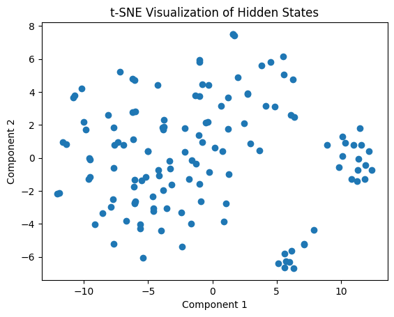
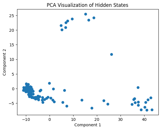
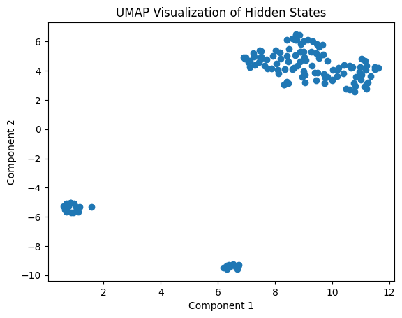
It’s always hard to know what this means. Let’s look at it in 3D (commented out on the blog but you can uncomment fig.show() and run it to see the results).
pca_3d = PCA(n_components=3)
hidden_states_pca_3d = pca_3d.fit_transform(hidden_states)

df = pd.DataFrame(hidden_states_pca_3d, columns=["Component 1", "Component 2", "Component 3"])

fig = px.scatter_3d(
    df,
    x="Component 1",
    y="Component 2",
    z="Component 3",
    color="Component 1",
    color_continuous_scale=px.colors.sequential.Plasma,
    size_max=10,
    opacity=0.8,
    template="plotly_dark",
    title="3D PCA Visualization of Hidden States",
    labels={
        "Component 1": "Component 1",
        "Component 2": "Component 2",
        "Component 3": "Component 3",
    },
    width=800,
    height=600,
)

# fig.show()
Doing it at Scale
Getting Hidden States
Now, we’re going to get all the hidden states. We’ll get the ones with positive sentiment and negative sentiment.
def get_encoder_hidden_states(model, tokenizer, input_text, layer=-1):
    """
    Given an encoder model and some text, gets the encoder hidden states (in a given layer, by default the last)
    on that input text (where the full text is given to the encoder).

    Returns a numpy array of shape (hidden_dim,)
    """
    # tokenize
    encoder_text_ids = tokenizer(input_text, truncation=True, return_tensors="pt").input_ids.to(model.device)

    # forward pass
    with torch.no_grad():
        output = model(encoder_text_ids, output_hidden_states=True)

    # get the appropriate hidden states
    hs_tuple = output["hidden_states"]

    hs = hs_tuple[layer][0, -1].detach().cpu().numpy()

    return hs
model.eval()
all_neg_hs, all_pos_hs, all_gt_labels = [], [], []
n = 100

for _ in tqdm(range(n)):
    # for simplicity, sample a random example until we find one that's a reasonable length
    # (most examples should be a reasonable length, so this is just to make sure)
    while True:
        idx = np.random.randint(len(data))
        text, true_label = data[idx]["content"], data[idx]["label"]
        # the actual formatted input will be longer, so include a bit of a margin
        if len(tokenizer(text)) < 400:
            break

    # get hidden states
    neg_hs = get_encoder_hidden_states(model, tokenizer, create_prompt_review(text, 0))
    pos_hs = get_encoder_hidden_states(model, tokenizer, create_prompt_review(text, 1))

    # collect
    all_neg_hs.append(neg_hs)
    all_pos_hs.append(pos_hs)
    all_gt_labels.append(true_label)

X_neg = np.stack(all_neg_hs)
X_pos = np.stack(all_pos_hs)
y = np.stack(all_gt_labels)
100%|█████████████████████████████████████████| 100/100 [00:16<00:00, 5.93it/s]
Now we have our hidden states. Let’s split them into train and test sets.
X_pos_train, X_pos_test, X_neg_train, X_neg_test, y_train, y_test = train_test_split(
    X_pos, X_neg, y, random_state=42
)
Test Model Representations
The question is, do we have good representations of the data? The way to check this is to make a simple model. If logistic regression can’t use the hidden states to classify the review, they’re not any good.
We want to combine the positive and negative together and there are a few ways we could do that. The simplest way is just to subtract them.
X_train = X_neg_train - X_pos_train
X_test = X_neg_test - X_pos_test
lr = LogisticRegression(class_weight="balanced")
lr.fit(X_train, y_train)
print(f"Logistic regression accuracy: {lr.score(X_test, y_test)}")
Logistic regression accuracy: 0.92
Yay! We’ve built good representations.
Contrast-Consistent Search
Now let’s use at Contrast-Consistent Search (CCS). You can learn more about it in the paper linked at the top.
The first step is to prepare the data by normalizing it and turning it into a Pytorch tensor.
def normalize(x: np.ndarray) -> np.ndarray:
    normalized_x = x - x.mean(axis=0, keepdims=True)
    return normalized_x
# Prepare data
X_neg_train_normed = normalize(X_neg_train)
X_pos_train_normed = normalize(X_pos_train)
def convert_to_tensors(x0: np.ndarray, x1: np.ndarray, device: str) -> tuple[torch.Tensor, torch.Tensor]:
    x0 = torch.tensor(x0, dtype=torch.float, device=device)
    x1 = torch.tensor(x1, dtype=torch.float, device=device)
    return x0, x1
# Convert data to tensors
X_neg_train_tensor, X_pos_train_tensor = convert_to_tensors(X_neg_train_normed, X_pos_train_normed, device="cuda")
Now we can train with CCS. Note that we don’t need any labels for this.
To do this, we’ll need to create a probe. A probe is a simple model used in self-supervised learning to learn a task-specific representation from the features extracted by an unsupervised model. In this case, the probe is a binary classifier that distinguishes between the two sets of samples.
def create_probe(input_size: int, device: str) -> nn.Module:
    probe = nn.Sequential(nn.Linear(input_size, 1), nn.Sigmoid())
    probe.to(device)
    return probe
probe = create_probe(X_neg_train_tensor.shape[-1], "cuda")
The loss function is a crucial component of the CCS algorithm because it serves as the primary driving force behind the optimization of the model’s parameters. In this specific case, the CCS algorithm aims to learn a binary classifier that can distinguish between two sets of samples.
The CCS loss function comprises two key components: the informative loss and the consistent loss. The informative loss encourages the model to minimize the squared difference between the probabilities assigned to the samples from both sets. This component of the loss function aims to make the model more discriminative, pushing it to assign higher probabilities to one set of samples and lower probabilities to the other set. In doing so, the model is encouraged to identify patterns or features that separate the two sets of samples, thus maximizing the information it can learn from the unlabeled data.
The consistent loss, on the other hand, focuses on ensuring that the model remains consistent in its predictions. This is achieved by penalizing the squared difference between the probabilities assigned to samples from x0 and the complement of the probabilities assigned to the corresponding samples from x1. By minimizing this component of the loss function, the model is encouraged to consistently assign complementary probabilities to samples from the two sets. This consistency is crucial for ensuring the model’s robustness and preventing it from overfitting to spurious correlations in the training data.
def get_loss(p0: torch.Tensor, p1: torch.Tensor) -> torch.Tensor:
    informative_loss = (torch.min(p0, p1) ** 2).mean(0)
    consistent_loss = ((p0 - (1 - p1)) ** 2).mean(0)
    return informative_loss + consistent_loss
We’ll write a function that finds the best probe and returns it.
def train(probe: nn.Module,
          x0: torch.Tensor,
          x1: torch.Tensor,
          num_epochs: int,
          lr: float,
          weight_decay: float,
          device: str) -> float:

    # Shuffle the input data
    permutation = torch.randperm(len(x0))
    x0, x1 = x0[permutation], x1[permutation]

    # Initialize the optimizer
    optimizer = torch.optim.AdamW(probe.parameters(), lr=lr, weight_decay=weight_decay)

    # Set batch size and number of batches
    batch_size = len(x0)
    nbatches = len(x0) // batch_size

    # Training loop
    for _ in range(num_epochs):
        for j in range(nbatches):
            # Create input batches
            x0_batch = x0[j * batch_size : (j + 1) * batch_size]
            x1_batch = x1[j * batch_size : (j + 1) * batch_size]

            # Forward pass through the probe
            p0, p1 = probe(x0_batch), probe(x1_batch)

            # Calculate loss
            loss = get_loss(p0, p1)

            # Update the probe's parameters
            optimizer.zero_grad()
            loss.backward()
            optimizer.step()

    return loss.detach().cpu().item()
def find_best_probe(
    probe: nn.Module,
    X_neg: torch.Tensor,
    X_pos: torch.Tensor,
    num_epochs: int,
    ntries: int,
    lr: float,
    weight_decay: float,
    device: str,
) -> tuple[nn.Module, float]:
    """
    Train the probe for multiple attempts and return the best probe and its loss.

    Parameters:
    probe: Initial probe model to train.
    X_neg: Negative class data.
    X_pos: Positive class data.
    num_epochs: Number of training epochs for each try.
    ntries: Number of attempts to find the best probe.
    lr: Learning rate for the optimizer.
    weight_decay: Weight decay for the optimizer.
    batch_size: Batch size for training, set to -1 for full batch training.
    device: Device to use for training, e.g. "cuda" or "cpu".

    Returns the best probe found and its corresponding loss.
    """
    best_loss = np.inf
    for _ in range(ntries):
        # Create and train a new probe for each attempt
        probe = create_probe(X_neg.shape[-1], device)
        loss = train(probe, X_neg, X_pos, num_epochs, lr, weight_decay, device)

        # Update the best probe if the current loss is lower
        if loss < best_loss:
            best_probe = copy.deepcopy(probe)
            best_loss = loss

    return best_probe, best_loss
best_probe, best_loss = find_best_probe(probe, X_neg_train_tensor, X_pos_train_tensor, num_epochs=1000, ntries=10, lr=1e-3,
                        weight_decay=0.01, device="cuda")
Now we can evaluate our results.
def get_acc(probe: nn.Module, X_neg_test: np.ndarray, X_pos_test: np.ndarray, y_test: np.ndarray, device: str) -> float:
    """
    Compute the accuracy of the probe on the given test data.

    Parameters:
    probe: The trained probe model.
    X_neg_test: Negative class test data.
    X_pos_test: Positive class test data.
    y_test: Test labels.
    device: Device to use for evaluation, e.g. "cuda" or "cpu".

    Returns the accuracy of the probe on the test data.
    """
    # Normalize the test data
    x0_test_normalized = normalize(X_neg_test)
    x1_test_normalized = normalize(X_pos_test)

    # Convert the test data to tensors
    x0_test, x1_test = convert_to_tensors(x0_test_normalized, x1_test_normalized, device)

    # Compute probabilities with the best probe
    with torch.no_grad():
        p0, p1 = probe(x0_test), probe(x1_test)

    # Compute average confidence and predictions
    avg_confidence = 0.5 * (p0 + (1 - p1))
    predictions = (avg_confidence.detach().cpu().numpy() < 0.5).astype(int)[:, 0]

    # Calculate the accuracy
    acc = (predictions == y_test).mean()
    acc = max(acc, 1 - acc)

    return acc
ccs_acc = get_acc(best_probe, X_neg_test, X_pos_test, y_test, device="cuda")
print(f"CCS accuracy: {ccs_acc}")
CCS accuracy: 0.84
The final accuracy is pretty good! This indicates that the algorithm is able to learn meaningful patterns from the given data without the need for explicit labels.