
Local Interpretable Model-agnostic Explanations (LIME) is an important technique for explaining the predictions of machine learning models. It is called “model-agnostic” because it can be used to explain any machine learning model, regardless of the model’s architecture or how it was trained. The key to LIME is to “zoom in” on a decision boundary and learn an interpretable model around that specific area. Then we can see exactly how various factors affect the decision boundary. In this post, I’ll show how to use LIME to explain an image classification model.
Table of Contents
import json

import matplotlib.pyplot as plt
import numpy as np
import torch
import torch.nn.functional as F
from lime.lime_image import LimeImageExplainer
from PIL import Image
from skimage.segmentation import mark_boundaries
from torchvision import models, transforms
from torchvision.models import Inception_V3_Weights
Load the Data
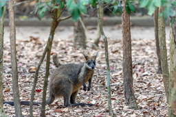
Let’s load an image that we’ll use our model to predict.
im_path = 'wallaby.jpg'
im = Image.open(im_path)
I’m going to resize it and then take a look at it.
im.thumbnail((256, 256), resample=Image.Resampling.LANCZOS)
im
Load the Model
Now let’s get our model. For simplicity, I’m going to use an off-the-shelf one: InceptionV3.
model = models.inception_v3(weights=Inception_V3_Weights.DEFAULT)
Set it to evaluation mode.
model.eval();
Prepare the Image
There are a few things we need to do to prepare the images. There’s nothing special here - just some stuff for working with a PyTorch model. For one, we’ll have to use the ImageNet mean and standard deviation to transform the image.
IMAGENET_MEAN = [0.485, 0.456, 0.406]
IMAGENET_STD = [0.229, 0.224, 0.225]
normalize = transforms.Normalize(mean=IMAGENET_MEAN, std=IMAGENET_STD)
transform = transforms.Compose([transforms.ToTensor(), normalize])
im_t = transform(im).unsqueeze(0)
with open("imagenet_class_index.json", "r") as f:
    imagenet_classes_dict = json.load(f)
imagenet_classes = [imagenet_classes_dict[str(i)][1] for i in range(len(imagenet_classes_dict))]
Classify the Image
logits = model(im_t)
probs = F.softmax(logits, dim=1)
pred = probs.topk(1)
pred_prob = pred.values[0][0].detach().numpy()
pred_index = pred.indices[0][0].numpy()
print(f"We predicted {imagenet_classes[pred_index]} with a probability of {pred_prob:.2%}.")
We predicted wallaby with a probability of 100.00%.
Explain the Predictions
Now we can use LIME to explain our predictions. We start by making an instance of a LimeImageExplainer.
explainer = LimeImageExplainer()
Next, we call the explain_instance method and pass it the image and the prediction. This method will return an explanation object, which contains the information about how the model made the prediction. We’ll need a batch_predict function to pass to it.
def batch_predict(images: list):
    """
    Generic batch prediction in PyTorch
    """
    model.eval()
    batch = torch.stack(tuple(transform(i) for i in images), dim=0)
    device = torch.device("cuda" if torch.cuda.is_available() else "cpu")
    model.to(device)
    batch = batch.to(device)
    logits = model(batch)
    probs = F.softmax(logits, dim=1)
    return probs.detach().cpu().numpy()
explain_instance takes several arguments. The top_labels parameter specifies the number of labels that the explanation should focus on. The hide_color parameter specifies whether the explanation should include color information. The num_samples parameter specifies the number of samples to use when approximating the model’s behavior.
explanation = explainer.explain_instance(np.array(im), batch_predict, top_labels=1, hide_color=0, num_samples=1000)
0%| | 0/1000 [00:00<?, ?it/s]
img, mask = explanation.get_image_and_mask(explanation.top_labels[0], positive_only=False)
img_boundry = mark_boundaries(img / 255.0, mask)
plt.imshow(img_boundry)
plt.tick_params(left=False, right=False, labelleft=False, labelbottom=False, bottom=False)
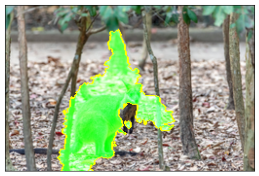
Now we can look at the areas of the image that are highlighted in the image. These are the regions that the model attended to when making the prediction. We can see that the area covering the wallaby is green, indicating that those areas were positively associated with the class “wallaby” in the image. This is one way we can make sure the model is looking at what we expect it to.
It’s also good to look at the weights that LIME assigns to each region. The weights indicate the relative importance of each region in the model’s prediction. Regions with higher weights were more important for the prediction, while regions with lower weights were less important.