This post is a tutorial demonstrating how to use Grad-CAM (Gradient-weighted Class Activation Mapping) for interpreting the output of a neural network. Grad-CAM is a visualization technique that highlights the regions a convolutional neural network (CNN) relied upon most to make predictions. While Grad-CAM is applicable to any CNN, it is predominantly employed with image classification models. This tutorial utilizes TensorFlow for implementation, but I made a parallel tutorial that works with PyTorch.

Table of Contents

• Load the Image
• Create a Model
• Preprocess the Image
• Predict the Top Class
• Determine the Target Layer
• Create Grad-CAM Model and Compute Heatmap
• Visualize the Heatmap

import json
import urllib.request
from typing import Optional

import cv2
import matplotlib.pyplot as plt
import numpy as np
import requests
import tensorflow as tf
from PIL import Image
from pyxtend import struct
from tensorflow.keras.applications.xception import Xception, decode_predictions, preprocess_input
from tensorflow.keras.preprocessing import image

Load the Image

We’ll pull the image from a remote URL so it’s easy to use.

IMAGE_URL = "https://raw.githubusercontent.com/jss367/files/main/cat_and_dog_hats.png"
img_path = 'cat_and_dog_hats.png'

with urllib.request.urlopen(IMAGE_URL) as response, open(img_path, "wb") as out_file:
    out_file.write(response.read())

input_image = Image.open(img_path)

input_image

This image has a few different objects in it, which might not be ideal for an image classification demo. But I’m going to use it so we can look at how to focus on specific classes within an image.

Create a Model

For this tutorial, I’m going to use Xception, but you can use any model.

model = Xception(weights="imagenet")

Preprocess the Image

Now that we have a model we can preprocess the image for the model.

def load_and_preprocess_image(img_path, img_size=(299, 299)):
    """
    (299, 299) is the default size for Xception
    """
    img = image.load_img(img_path, target_size=img_size)
    array = image.img_to_array(img)
    array = np.expand_dims(array, axis=0)
    return preprocess_input(array)

preprocessed_input = load_and_preprocess_image(img_path)

Predict the Top Class

Now let’s make a prediction.

predictions = model.predict(preprocessed_input)

1/1 [==============================] - 1s 781ms/step

struct(predictions)

{'ndarray': ['float32, shape=(1, 1000)']}

The prediction is a numpy array of values. To understand the predictions, we’ll have to use Xception’s decode_predictions function. Let’s look at the top 10 predictions.

pred_class_idx = np.argmax(predictions)
decoded_predictions = decode_predictions(predictions, top=10)[0]
decoded_predictions

[('n02100583', 'vizsla', 0.17101629),
 ('n02087394', 'Rhodesian_ridgeback', 0.14642362),
 ('n02108089', 'boxer', 0.031510208),
 ('n02108422', 'bull_mastiff', 0.030151485),
 ('n02090379', 'redbone', 0.024255073),
 ('n02088466', 'bloodhound', 0.021224905),
 ('n02109047', 'Great_Dane', 0.01767018),
 ('n02099712', 'Labrador_retriever', 0.017465966),
 ('n03724870', 'mask', 0.012718478),
 ('n03494278', 'harmonica', 0.009038365)]

We can also get the id associated with the top prediction.

We can download the class labels to see what this correspond to.

IMAGENET_CLASSES_URL = "https://raw.githubusercontent.com/jss367/files/main/imagenet_classes.json"
class_labels = json.loads(requests.get(IMAGENET_CLASSES_URL).text)
struct(class_labels, examples=True)

{'list': ['tench', 'goldfish', 'great white shark', '...1000 total']}

predicted_class_name = class_labels[pred_class_idx]
print(f"Predicted class: {predicted_class_name} (index: {pred_class_idx}, probability: {decoded_predictions[0][2]:.2%})")

Predicted class: Vizsla (index: 211, probability: 17.10%)

Determine the Target Layer

OK, now we have predictions. Now we have to create a model that outputs the activations of the last convolutional layer as well as the output predictions.

We should use the last convolutional layer for Grad-CAM because it provides the highest level of spatial information before the model becomes spatially invariant. We don’t know the name of the last convolutional layer and unfortunately, we can’t just loop through them and look for if isinstance(layer, tf.keras.layers.Conv2D) because many convolutional layers are not instances of tf.keras.layers.Conv2D. Instead, we can print out all the layer names and look for the last one before a flatten or avg_pool layer. We know it’s going to be one of the last layers, so we’ll only print out the last ten.

[l.name for l in model.layers[-10:]]

['batch_normalization_3',
 'add_11',
 'block14_sepconv1',
 'block14_sepconv1_bn',
 'block14_sepconv1_act',
 'block14_sepconv2',
 'block14_sepconv2_bn',
 'block14_sepconv2_act',
 'avg_pool',
 'predictions']

Looks like block14_sepconv2_act is what we’re looking for.

last_conv_layer_name = 'block14_sepconv2_act'

Create Grad-CAM Model and Compute Heatmap

Now let’s create a Grad-CAM model

gradcam_model = tf.keras.models.Model([model.inputs], [model.get_layer(last_conv_layer_name).output, model.output])

Now we have to calculate the gradient of the class output with respect to the convolutional layer output. We’ll use the predicted class from the full model that we found before.

with tf.GradientTape() as tape:
    last_conv_layer_output, predictions = gradcam_model(preprocessed_input)
    loss = predictions[:, pred_class_idx]

Get the gradient of the output neuron with respect to the convolutional layer output.

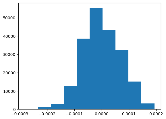
grads = tape.gradient(loss, last_conv_layer_output)

Let’s look at these gradients.

plt.hist(grads.numpy().flatten());

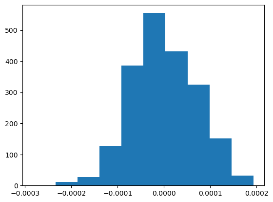
Now let’s average the gradient over all the channels in the convolutional layer output.

pooled_grads = tf.reduce_mean(grads, axis=(0, 1, 2))

plt.hist(pooled_grads.numpy().flatten());

Now we can compute the weighted sum of the convolutional layer output with respect to the averaged gradient. But first, we have to prepare the last_conv_layer_output. last_conv_layer_output is a 4D tensor with shape (batch_size, height, width, channels). We’ll take the first batch to reduce it to a 3D tensor.

last_conv_layer_output_3d = last_conv_layer_output[0]

Now we compute the dot product of last_conv_layer_output_3d and pooled_grads (with a new axis added to pooled_grads), which essentially performs a weighted sum of the feature maps in last_conv_layer_output_3d using the weights in pooled_grads.

heatmap = last_conv_layer_output @ pooled_grads[..., tf.newaxis]
heatmap = tf.squeeze(heatmap)

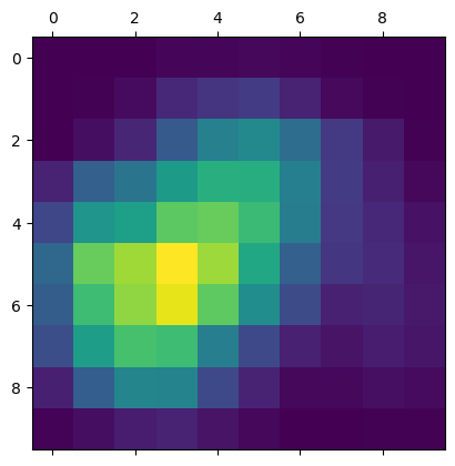
Then normalize the heatmap to values between 0 and 1 to make it easier to visualize.

heatmap = tf.maximum(heatmap, 0) / tf.math.reduce_max(heatmap)
heatmap = heatmap.numpy()

Now let’s take a look at what we’ve got.

plt.matshow(heatmap);

Visualize the Heatmap

That’s good. We’ve got a bit of work to do to display this though. We’ve got to resize, smooth, and overlay it on the original image so that we can really understand it. We’ll create a function to do that now.

def visualize_heatmap(img_path: str, heatmap: np.ndarray) -> None:
    # Read the image from the given file path
    img = cv2.imread(img_path)
    
    # Resize the heatmap to match the size of the original image
    heatmap = cv2.resize(heatmap, (img.shape[1], img.shape[0]))
    
    # Normalize the heatmap values to the range [0, 255] and cast to uint8
    heatmap = np.uint8(255 * heatmap)
    
    # Apply the JET colormap to the heatmap
    heatmap = cv2.applyColorMap(heatmap, cv2.COLORMAP_JET)
    
    # Blend the original image with the heatmap (60% original, 40% heatmap)
    superimposed_img = cv2.addWeighted(img, 0.6, heatmap, 0.4, 0)

    # Display the blended image in RGB format
    plt.imshow(cv2.cvtColor(superimposed_img, cv2.COLOR_BGR2RGB))
    plt.axis('off')
    plt.show()

visualize_heatmap(img_path, heatmap)

Let’s put it all into a function. But I want to make one more change. We previously only showed the heatmap for the predicted class. Now I want to allow it to show the heatmap for any class we specify. Below are some relevant ImageNet class indexes that we can look for. You can get the full list here.

GOOSE_INDEX = 99
VIZSLA_INDEX = 211
GERMAN_SHEPARD_INDEX = 235
GREAT_DANE_INDEX = 246
CHOW_INDEX = 260
TABBY_CAT_INDEX = 281
TIGER_CAT_INDEX = 282
EGYPTIAN_CAT_INDEX = 285
COWBOY_HAT_INDEX = 515

def grad_cam(
    model: tf.keras.Model, preprocessed_input: np.ndarray, layer_name: str, class_index: Optional[int] = None
) -> np.ndarray:
    """
    Generate a Grad-CAM heatmap for a specific class index or the top prediction.

    Args:
        model: The trained model.
        preprocessed_input: The input image after pre-processing.
        layer_name: The name of the target convolutional layer.
        class_index: The target class index. If None, the top prediction is used. Defaults to None.

    Returns the generated Grad-CAM heatmap.
    """

    if not class_index:
        # Use the top prediction
        class_index = np.argmax(model.predict(preprocessed_input))

    # Get the target convolutional layer
    target_conv_layer = model.get_layer(layer_name)

    # Create a model using the target layer's output and the original model's output
    gradcam_model = tf.keras.models.Model([model.inputs], [model.get_layer(layer_name).output, model.output])

    # Record operations for automatic differentiation
    with tf.GradientTape() as tape:
        layer_output, predictions = gradcam_model(preprocessed_input)
        loss = predictions[:, class_index]

    # Compute the gradient of the loss with respect to the layer output
    grads = tape.gradient(loss, layer_output)
    # Compute the average gradient for each feature map
    pooled_grads = tf.reduce_mean(grads, axis=(0, 1, 2))

    # Select the first instance (assuming batch size is 1) from the layer output
    layer_output_single_instance = layer_output[0]

    # Compute the weighted sum of the layer output using pooled_grads as weights
    heatmap = layer_output_single_instance @ pooled_grads[..., tf.newaxis]
    heatmap = tf.squeeze(heatmap)
    # Normalize the heatmap between 0 and 1
    heatmap = tf.maximum(heatmap, 0) / tf.math.reduce_max(heatmap)
    heatmap = heatmap.numpy()

    return heatmap

heatmap = grad_cam(model, preprocessed_input, last_conv_layer_name)
visualize_heatmap(img_path, heatmap)

1/1 [==============================] - 0s 109ms/step

heatmap = grad_cam(model, preprocessed_input, last_conv_layer_name, EGYPTIAN_CAT_INDEX)
visualize_heatmap(img_path, heatmap)

heatmap = grad_cam(model, preprocessed_input, last_conv_layer_name, COWBOY_HAT_INDEX)
visualize_heatmap(img_path, heatmap)