
In this post I want to talk about some techniques for dealing with skewed data, especially left-skewed data. Left-skewed data is a bit of a rarity. It’s something you don’t see very often, kind of like a left-handed unicorn. It can also be difficult to work with if you’re not prepared.
Table of Contents
import matplotlib.pyplot as plt
import numpy as np
import pandas as pd
from scipy.stats import skewtest
from sklearn.datasets import load_breast_cancer
Let’s load some data from the breast cancer dataset.
data = load_breast_cancer()

feature_df = pd.DataFrame(data.data, columns=data.feature_names)
label_df = pd.DataFrame(data.target).rename(columns={0: "Diagnosis"})

df = pd.concat([feature_df, label_df], axis=1)
df.head()
| mean radius | mean texture | mean perimeter | mean area | mean smoothness | mean compactness | mean concavity | mean concave points | mean symmetry | mean fractal dimension | ... | worst texture | worst perimeter | worst area | worst smoothness | worst compactness | worst concavity | worst concave points | worst symmetry | worst fractal dimension | Diagnosis | |
|---|---|---|---|---|---|---|---|---|---|---|---|---|---|---|---|---|---|---|---|---|---|
| 0 | 17.99 | 10.38 | 122.80 | 1001.0 | 0.11840 | 0.27760 | 0.3001 | 0.14710 | 0.2419 | 0.07871 | ... | 17.33 | 184.60 | 2019.0 | 0.1622 | 0.6656 | 0.7119 | 0.2654 | 0.4601 | 0.11890 | 0 |
| 1 | 20.57 | 17.77 | 132.90 | 1326.0 | 0.08474 | 0.07864 | 0.0869 | 0.07017 | 0.1812 | 0.05667 | ... | 23.41 | 158.80 | 1956.0 | 0.1238 | 0.1866 | 0.2416 | 0.1860 | 0.2750 | 0.08902 | 0 |
| 2 | 19.69 | 21.25 | 130.00 | 1203.0 | 0.10960 | 0.15990 | 0.1974 | 0.12790 | 0.2069 | 0.05999 | ... | 25.53 | 152.50 | 1709.0 | 0.1444 | 0.4245 | 0.4504 | 0.2430 | 0.3613 | 0.08758 | 0 |
| 3 | 11.42 | 20.38 | 77.58 | 386.1 | 0.14250 | 0.28390 | 0.2414 | 0.10520 | 0.2597 | 0.09744 | ... | 26.50 | 98.87 | 567.7 | 0.2098 | 0.8663 | 0.6869 | 0.2575 | 0.6638 | 0.17300 | 0 |
| 4 | 20.29 | 14.34 | 135.10 | 1297.0 | 0.10030 | 0.13280 | 0.1980 | 0.10430 | 0.1809 | 0.05883 | ... | 16.67 | 152.20 | 1575.0 | 0.1374 | 0.2050 | 0.4000 | 0.1625 | 0.2364 | 0.07678 | 0 |
5 rows × 31 columns
Let’s run a skewtest on the data to see how skewed it is.
skew_results = skewtest(df)
skew_results
SkewtestResult(statistic=array([ 7.9622136 ,  5.88215201,  8.27259482, 11.74893638,  4.290775  ,
        9.46629397, 10.59171403,  9.35871813,  6.45269024, 10.09216315,
       16.58088149, 11.75210248, 17.44633464, 21.14164598, 14.32036053,
       12.82429991, 20.62412273, 10.80823381, 13.91279644, 18.49190706,
        8.96247615,  4.64939677,  9.11009444, 12.65331114,  3.93417231,
       10.9492919 ,  9.23843169,  4.60113196, 10.75517885, 11.82359913,
       -4.90193592]), pvalue=array([1.68988430e-15, 4.04966147e-09, 1.31074540e-16, 7.15132884e-32,
       1.78050645e-05, 2.89948577e-21, 3.25574965e-26, 8.07099084e-21,
       1.09881815e-10, 5.98361587e-24, 9.58130444e-62, 6.88833407e-32,
       3.67043537e-68, 3.29387877e-99, 1.63273983e-46, 1.19864358e-37,
       1.66727337e-94, 3.14670056e-27, 5.29673293e-44, 2.39917722e-76,
       3.17467671e-19, 3.32907258e-06, 8.23102934e-20, 1.07257301e-36,
       8.34838797e-05, 6.69690805e-28, 2.50136485e-20, 4.20201106e-06,
       5.60252308e-27, 2.94779180e-32, 9.48967940e-07]))
It’s mostly right skewed. Only one is left skewed (the negative value).
Right-skewed Data
There are lots of ways to deal with right-skewed data, so let’s start there. Let’s work with the most skewed example.
right_skewed_index = np.argmax(skew_results.statistic)
max_skewed_name = df.iloc[:, right_skewed_index].name
max_skewed_name
'area error'
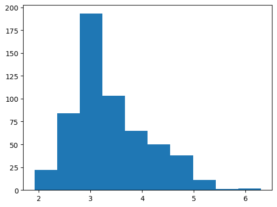
right_skewed_data = df[max_skewed_name]
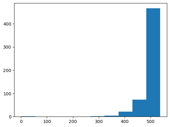
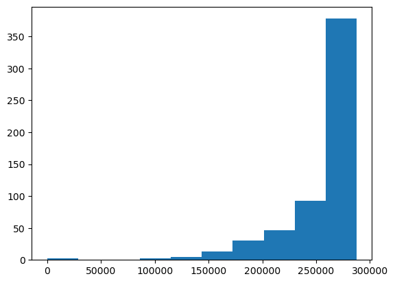
plt.hist(right_skewed_data);

That’s a nice right-skewed distribution. Many machine learning techniques have difficulty modeling such distributions. However, certain models like mixture density networks are able to handle arbitrary distributions by using a combination of multiple probability distributions. Additionally, there are models such as tree-based models, like Random Forest, XGBoost and LightGBM, which are not affected by the distribution of the data, and can model the data directly. These models are considered as non-parametric models, they don’t assume a specific distribution of the data and they can capture complex non-linear relationship in the data.
However, the simplest thing to do is often to transform the data so that it is normally distributed.
Transforming Right-skewed data
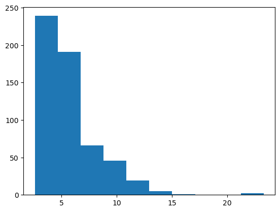
My first approach is to take the log. This is often all you need.
plt.hist(np.log(right_skewed_data));
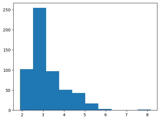
Although you can also use the square root.
plt.hist(np.sqrt(right_skewed_data));
If the dataset has outliers that are really far away that you don’t want to remove, you might think about taking the cubic root. This data is so highly skewed that it might work pretty well.
plt.hist(np.cbrt(right_skewed_data));
Nice! I would still go with np.log but this would work as well.
Left-skewed Data
OK, now let’s look at the left-skewed data. Though you might think the same techniques would apply, this isn’t the case.
Let’s look at our skewtest results again.
skew_results.statistic
array([ 7.9622136 ,  5.88215201,  8.27259482, 11.74893638,  4.290775  ,
        9.46629397, 10.59171403,  9.35871813,  6.45269024, 10.09216315,
       16.58088149, 11.75210248, 17.44633464, 21.14164598, 14.32036053,
       12.82429991, 20.62412273, 10.80823381, 13.91279644, 18.49190706,
        8.96247615,  4.64939677,  9.11009444, 12.65331114,  3.93417231,
       10.9492919 ,  9.23843169,  4.60113196, 10.75517885, 11.82359913,
       -4.90193592])
left_skewed_index = np.argmin(skew_results.statistic)
df.iloc[:, left_skewed_index].name
'Diagnosis'
Oh. The “left-skewed” data is the label. This probably isn’t what we’re looking for. Let’s plot it anyway.
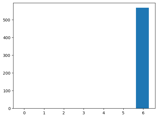
df.iloc[:, left_skewed_index].plot.hist();
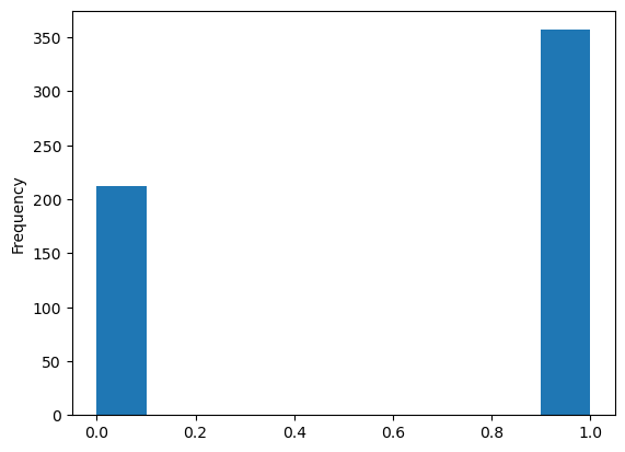
OK, you can see why it showed up as left-skewed in the test, but this just goes to show why it’s important to actually look at the histogram and not only a skewness test. So in this entire dataset, there isn’t a single example of a left-skewed feature. This goes back to what I was saying about it being less common.
I think the best thing to do is just make some left-skewed data for our current dataset. This is a bit of a spoiler for the final answer, but, oh well.
We can flip the skew by throwing a minus sign in front of the data. I also add the max value to keep the numbers positive, and an addition 1 to keep everything at least 1 (in case I need to log transform it later). So the final flip ends up looking like this:
left_skewed_data = 1 + int(right_skewed_data.max()) - right_skewed_data
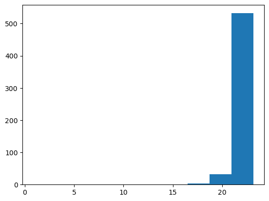
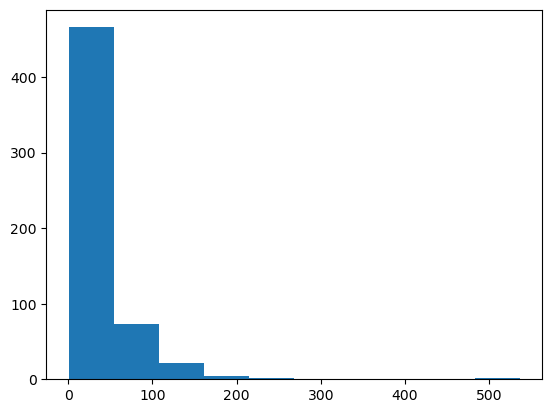
plt.hist(left_skewed_data);
There we go! The mythical left-skewed data! (I swear you do see it in real life sometimes.)
Transforming Left-skewed data
Let’s try the transforms as before.
plt.hist(np.log(left_skewed_data));
Wow, that looks awful. Let’s try another.
plt.hist(np.sqrt(left_skewed_data));
Still worse than the original.
OK, why don’t we try the reverse? If log and sqrt don’t work, what about exp and square?
plt.hist(np.exp(left_skewed_data));
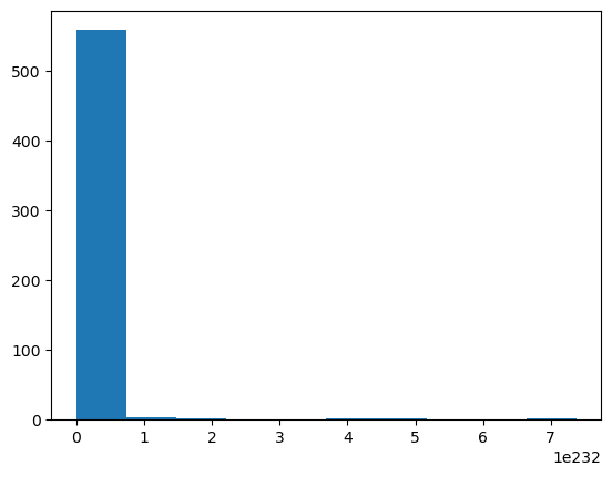
It’s… somehow the opposite yet the worst of all? Note the scale is 1e232.
plt.hist(np.square(left_skewed_data));
At least that’s not abominable! It’s still distinctly left-skewed, but at least it still looks like something.
So what’s the solution here? As you might have guessed from how we got the data, the best solution is to throw a negative sign in front of it (and do the other steps) so that’s it’s right-skewed. Then you can treat it as normal right-skewed data. As we saw before, switching the skew looks like this:
right_skewed_data = 1 + int(left_skewed_data.max()) - left_skewed_data
plt.hist(right_skewed_data);
There we go. There’s our right-skewed data back. From here we can do any of the techniques described earlier.