This post is a tutorial demonstrating how to use Grad-CAM (Gradient-weighted Class Activation Mapping) for interpreting the output of a neural network. Grad-CAM is a visualization technique that highlights the regions a convolutional neural network (CNN) relied upon most to make predictions. While Grad-CAM is applicable to any CNN, it is predominantly employed with image classification models. This tutorial utilizes PyTorch for implementation, but I made a parallel tutorial that works with TensorFlow.

Table of Contents

import json
import urllib.request

import cv2
import matplotlib.pyplot as plt
import numpy as np
import requests
import torch
import torch.nn as nn
import torchvision.models as models
import torchvision.transforms as transforms
from PIL import Image
from pyxtend import struct
from torchvision.models.resnet import ResNet18_Weights

Load the Image

We’ll pull the image from a remote URL so it’s easy to use.

IMAGE_URL = "https://raw.githubusercontent.com/jss367/files/main/cat_and_dog_hats.png"
img_path = 'cat_and_dog_hats.png'

with urllib.request.urlopen(IMAGE_URL) as response, open(img_path, "wb") as out_file:
    out_file.write(response.read())

input_image = Image.open(img_path)

input_image

png

This image has a few different objects in it, which might not be ideal for an image classification demo. But I’m going to use it so we can look at how to focus on specific classes within an image.

Create a Model

For this tutorial, we will use a pre-trained ResNet-18 model, but you can use any other pre-trained model. Make sure that the model is in evaluation mode.

model = models.resnet18(weights=ResNet18_Weights.DEFAULT)
model.eval();

Preprocess the Image

Define the input transformation pipeline, which will be applied to the input image:

IMAGENET_MEAN_VALUES = [0.485, 0.456, 0.406]
IMAGENET_STD_VALUES = [0.229, 0.224, 0.225]

preprocess = transforms.Compose(
    [
        transforms.Resize((224, 224)),
        transforms.ToTensor(),
        transforms.Normalize(mean=IMAGENET_MEAN_VALUES, std=IMAGENET_STD_VALUES),
    ]
)

Apply pre-processing and convert it into a batch of size 1.

input_tensor = preprocess(input_image)
input_batch = input_tensor.unsqueeze(0)

Predict the Top Class

Now let’s make a prediction.

logits = model(input_batch)

struct(logits)

{'Tensor': ['torch.float32, shape=(1, 1000)']}

probs = torch.softmax(logits, dim=1)
pred_class_idx = torch.argmax(probs, dim=1).item()
predicted_prob = probs[0, pred_class_idx].item()

We can download the class labels to see what this corresponds to.

IMAGENET_CLASSES_URL = "https://raw.githubusercontent.com/jss367/files/main/imagenet_classes.json"
class_labels = json.loads(requests.get(IMAGENET_CLASSES_URL).text)
struct(class_labels, examples=True)

{'list': ['tench', 'goldfish', 'great white shark', '...1000 total']}

predicted_class_name = class_labels[pred_class_idx]
print(f"Predicted class: {predicted_class_name} (index: {pred_class_idx}, probability: {predicted_prob:.2%})")

Predicted class: cowboy hat (index: 515, probability: 61.57%)

Determine the Target Layer

OK, now we have predictions. Now we have to create a model that outputs the activations of the last convolutional layer as well as the output predictions.

We should use the last convolutional layer for Grad-CAM because it provides the highest level of spatial information before the model becomes spatially invariant. Now we can loop through them and look for if isinstance(layer, nn.Conv2d).

def find_last_conv_layer(model: nn.Module) -> tuple:
    last_conv_layer_name = None
    last_conv_layer = None

    for layer_name, layer in model.named_modules():
        if isinstance(layer, nn.Conv2d):
            last_conv_layer_name = layer_name
            last_conv_layer = layer

    return last_conv_layer_name, last_conv_layer

layer_name, target_layer = find_last_conv_layer(model)
print(layer_name)

layer4.1.conv2

Create Grad-CAM Model

Define the Grad-CAM class, which will store the gradients and activations of the target layer and compute the Grad-CAM heatmap.

class GradCAM:
    def __init__(self, model, target_layer):
        self.model = model
        self.target_layer = target_layer
        self.gradients = None
        self.activations = None

        # Register hooks for gradients and activations
        target_layer.register_forward_hook(self.forward_hook)
        target_layer.register_full_backward_hook(self.full_backward_hook)

    def forward_hook(self, module, input, output):
        self.activations = output.detach()

    def full_backward_hook(self, module, grad_input, grad_output):
        self.gradients = grad_output[0].detach()

    def compute_heatmap(self, input_batch, class_idx=None):
        # Forward pass
        logits = self.model(input_batch)
        self.model.zero_grad()

        if class_idx is None:
            class_idx = torch.argmax(logits, dim=1).item()

        # Compute gradients for the target class
        one_hot_output = torch.zeros_like(logits)
        one_hot_output[0, class_idx] = 1
        logits.backward(gradient=one_hot_output)

        # Compute Grad-CAM heatmap
        weights = torch.mean(self.gradients, dim=[2, 3], keepdim=True)
        heatmap = torch.sum(weights * self.activations, dim=1, keepdim=True)
        heatmap = torch.relu(heatmap)  # ReLU removes negative values
        heatmap /= torch.max(heatmap)  # Normalize to [0, 1]

        # Get the predicted class probability
        probs = torch.softmax(logits, dim=1)
        predicted_prob = probs[0, class_idx].item()

        return heatmap.squeeze().cpu().numpy(), class_idx, predicted_prob

Create Grad-CAM Model and Compute Heatmap

Create an instance of the Grad-CAM class, specifying the target layer, and compute the heatmap for the input image.

gradcam = GradCAM(model, target_layer)

heatmap, predicted_class_idx, predicted_prob = gradcam.compute_heatmap(input_batch)

predicted_class_name = class_labels[predicted_class_idx]
print(f"Predicted class: {predicted_class_name} (index: {predicted_class_idx}, probability: {predicted_prob:.2%})")

Predicted class: cowboy hat (index: 515, probability: 61.57%)

Visualize the Heatmap

That’s good. We’ve got a bit of work to do to display this though. We’ve got to resize, smooth, and overlay it on the original image so that we can really understand it. We’ll create a function to do that now.

def visualize_heatmap(img_path: str, heatmap: np.ndarray) -> None:
    # Read the image from the given file path
    img = cv2.imread(img_path)
    
    # Resize the heatmap to match the size of the original image
    heatmap = cv2.resize(heatmap, (img.shape[1], img.shape[0]))
    
    # Normalize the heatmap values to the range [0, 255] and cast to uint8
    heatmap = np.uint8(255 * heatmap)
    
    # Apply the JET colormap to the heatmap
    heatmap = cv2.applyColorMap(heatmap, cv2.COLORMAP_JET)
    
    # Blend the original image with the heatmap (60% original, 40% heatmap)
    superimposed_img = cv2.addWeighted(img, 0.6, heatmap, 0.4, 0)

    # Display the blended image in RGB format
    plt.imshow(cv2.cvtColor(superimposed_img, cv2.COLOR_BGR2RGB))
    plt.axis('off')
    plt.show()

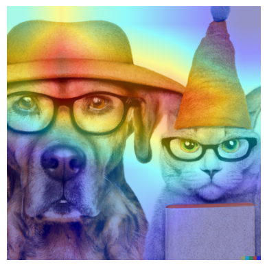
visualize_heatmap(img_path, heatmap)

png

We previously only showed the heatmap for the predicted class. Now I want to allow it to show the heatmap for any class we specify. Below are some relevant ImageNet class indexes that we can look for. You can get the full list here.

GOOSE_INDEX = 99
VIZSLA_INDEX = 211
GERMAN_SHEPARD_INDEX = 235
GREAT_DANE_INDEX = 246
CHOW_INDEX = 260
TABBY_CAT_INDEX = 281
TIGER_CAT_INDEX = 282
EGYPTIAN_CAT_INDEX = 285
COWBOY_HAT_INDEX = 515

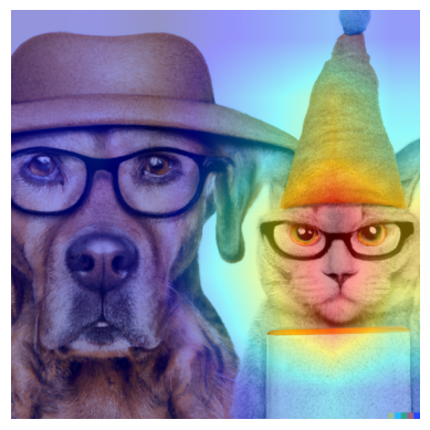
heatmap, predicted_class_idx, predicted_prob = gradcam.compute_heatmap(input_batch, VIZSLA_INDEX)
visualize_heatmap(img_path, heatmap)

png

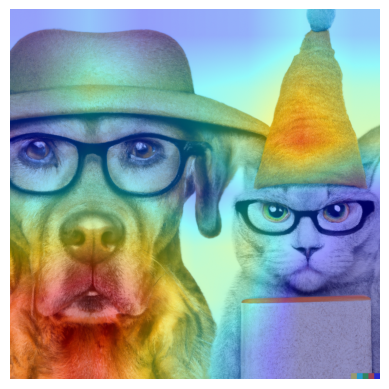
heatmap, predicted_class_idx, predicted_prob = gradcam.compute_heatmap(input_batch, EGYPTIAN_CAT_INDEX)
visualize_heatmap(img_path, heatmap)

png

Julius' Data Science Blog

Model Explainability with Grad-CAM in PyTorch