
In this notebook, we’ll demonstrate some data exploration techniques using the famous iris dataset. In the second notebook, we’ll use this data set to visualize a bunch of machine learning algorithms.
Table of Contents

import seaborn as sns
sns.set(style="dark")
import matplotlib.pyplot as plt
Load the Data
Load the data using seaborn. The dataset is also available from Scikit-learn and Keras, but it loads as a pandas DataFrame from seaborn, saving a step.
df = sns.load_dataset("iris")
Explore
Let’s look at what features are in the data set.
df.head()
| sepal_length | sepal_width | petal_length | petal_width | species | |
|---|---|---|---|---|---|
| 0 | 5.1 | 3.5 | 1.4 | 0.2 | setosa |
| 1 | 4.9 | 3.0 | 1.4 | 0.2 | setosa |
| 2 | 4.7 | 3.2 | 1.3 | 0.2 | setosa |
| 3 | 4.6 | 3.1 | 1.5 | 0.2 | setosa |
| 4 | 5.0 | 3.6 | 1.4 | 0.2 | setosa |
Then check how many of each species is recorded.
df['species'].value_counts()
setosa        50
versicolor    50
virginica     50
Name: species, dtype: int64
And let’s see what types of values are in the dataset and do some basic statistics on the set.
df.info()
<class 'pandas.core.frame.DataFrame'>
RangeIndex: 150 entries, 0 to 149
Data columns (total 5 columns):
 #   Column        Non-Null Count  Dtype
---  ------        --------------  -----
 0   sepal_length  150 non-null    float64
 1   sepal_width   150 non-null    float64
 2   petal_length  150 non-null    float64
 3   petal_width   150 non-null    float64
 4   species       150 non-null    object
dtypes: float64(4), object(1)
memory usage: 6.0+ KB
df.describe()
| sepal_length | sepal_width | petal_length | petal_width | |
|---|---|---|---|---|
| count | 150.000000 | 150.000000 | 150.000000 | 150.000000 |
| mean | 5.843333 | 3.057333 | 3.758000 | 1.199333 |
| std | 0.828066 | 0.435866 | 1.765298 | 0.762238 |
| min | 4.300000 | 2.000000 | 1.000000 | 0.100000 |
| 25% | 5.100000 | 2.800000 | 1.600000 | 0.300000 |
| 50% | 5.800000 | 3.000000 | 4.350000 | 1.300000 |
| 75% | 6.400000 | 3.300000 | 5.100000 | 1.800000 |
| max | 7.900000 | 4.400000 | 6.900000 | 2.500000 |
Fortunately, the data set is really clean so we can jump right into visualization.
Visualize
Let’s see how the different categories compare with each other.
hue_order = df['species'].unique()[::-1]
palette = sns.color_palette('bright')
sns.pairplot(df, hue="species", hue_order=hue_order, palette=palette, markers=["o", "s", "D"], diag_kind='kde');
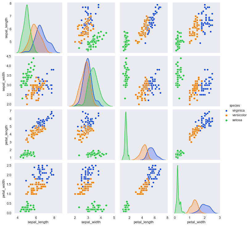
Nothing looks noticeably wrong with the data, and there aren’t any outliers that would confound a model.
Petal length and petal width appear to be good variables to distinguish the species, especially setosa. Let’s take a closer look at those.
sns.FacetGrid(df, hue='species', hue_order=hue_order, palette=palette, height=8) \
    .map(plt.scatter, 'petal_length','petal_width') \
    .add_legend();
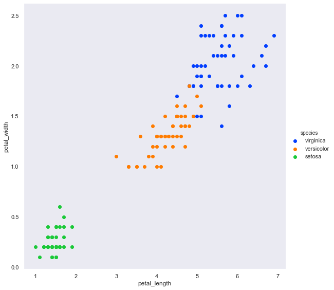
OK, it will be very easy to extract the setosa from the others.
Let’s see what the best way to separate versicolor from virginica is. We’ll create a new dataframe with just the two we’re focusing on.
# Exclude setosa
vvdf = df[df['species'] != 'setosa']
sns.pairplot(vvdf, hue="species", hue_order=hue_order, palette=palette, diag_kind='kde');
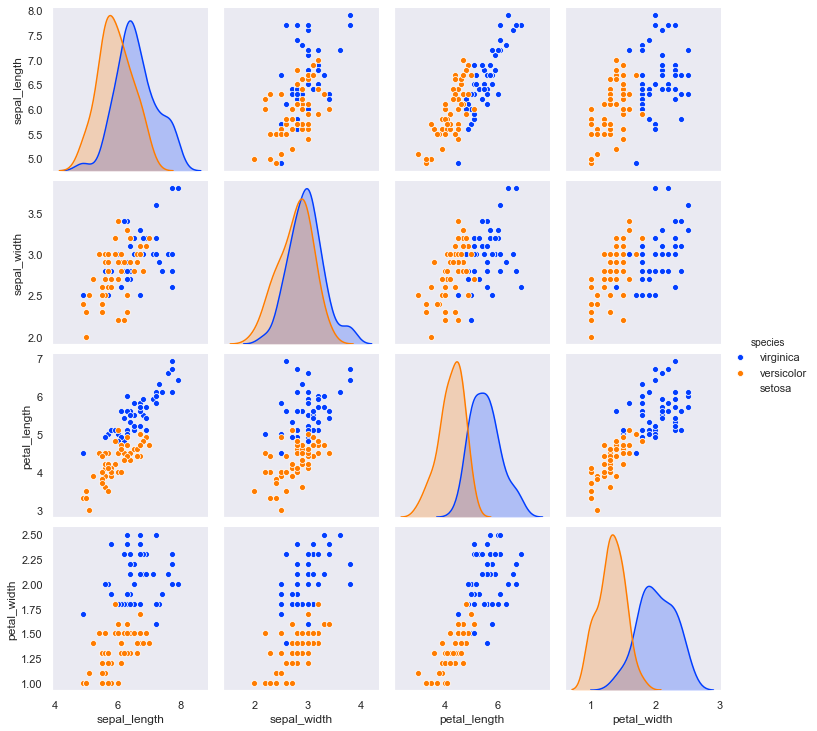
OK, these are not as easy to separate. We may have to do the best that we can. In Part II, we’ll look at how we can use machine learning models to analyze the data.