This post shows some of the various tools in Python for visualizing images. There are usually two steps to the visualization process. First, you’ll need to read in the image from a file path, usually as a numpy array or something similar. Then, you can visualize it with various libraries.
Table of Contents
Libraries
There are many libraries in Python to help with loading and processing images. Let’s look at a few of them.
from pyxtend import struct
from matplotlib import pyplot as plt
ImageIO
ImageIO is nice because it has a common interface for different image types.
import imageio
import numpy as np
image_path = '../roo.jpg'
img_arr = imageio.v2.imread(image_path)
struct(img_arr)
{'ndarray': ['uint8, shape=(256, 192, 3)']}
type(img_arr)
numpy.ndarray
isinstance(img_arr, np.ndarray)
True
As you can see, imageio.core.util.Array is a NumPy ndarray.
Time Test
%timeit img_arr = imageio.v2.imread(image_path)
877 µs ± 23.9 µs per loop (mean ± std. dev. of 7 runs, 1,000 loops each)
SKImage
SKImage is used for turning an image on disk into a numpy array, like so.
import skimage
from skimage.io import imread
image_path = '../roo.jpg'
skimage_read = imread(image_path)
skimage_read
array([[[232, 236, 245],
        [232, 236, 245],
        [232, 236, 245],
        ...,
        [227, 232, 236],
        [227, 232, 236],
        [227, 232, 236]],

       [[232, 236, 245],
        [232, 236, 245],
        [232, 236, 245],
        ...,
        [227, 232, 236],
        [227, 232, 236],
        [227, 232, 236]],

       [[232, 236, 245],
        [232, 236, 245],
        [232, 236, 245],
        ...,
        [227, 232, 236],
        [227, 232, 236],
        [227, 232, 236]],

       ...,

       [[128, 140,  58],
        [126, 138,  56],
        [123, 135,  53],
        ...,
        [106, 123,  31],
        [104, 121,  29],
        [103, 120,  28]],

       [[124, 136,  54],
        [122, 134,  52],
        [119, 131,  49],
        ...,
        [102, 122,  27],
        [ 99, 119,  24],
        [ 98, 118,  23]],

       [[121, 133,  51],
        [119, 131,  49],
        [116, 128,  46],
        ...,
        [101, 121,  26],
        [ 98, 118,  23],
        [ 96, 116,  21]]], dtype=uint8)
struct(skimage_read)
{'ndarray': ['uint8, shape=(256, 192, 3)']}
Time Test
%timeit skimage_read = imread(image_path)
901 µs ± 18.6 µs per loop (mean ± std. dev. of 7 runs, 1,000 loops each)
PyTorch
from torchvision.io import read_image
torch_read = read_image(image_path)
torch_read
tensor([[[232, 232, 232,  ..., 227, 227, 227],
         [232, 232, 232,  ..., 227, 227, 227],
         [232, 232, 232,  ..., 227, 227, 227],
         ...,
         [128, 126, 123,  ..., 106, 104, 103],
         [124, 122, 119,  ..., 102,  99,  98],
         [121, 119, 116,  ..., 101,  98,  96]],

        [[236, 236, 236,  ..., 232, 232, 232],
         [236, 236, 236,  ..., 232, 232, 232],
         [236, 236, 236,  ..., 232, 232, 232],
         ...,
         [140, 138, 135,  ..., 123, 121, 120],
         [136, 134, 131,  ..., 122, 119, 118],
         [133, 131, 128,  ..., 121, 118, 116]],

        [[245, 245, 245,  ..., 236, 236, 236],
         [245, 245, 245,  ..., 236, 236, 236],
         [245, 245, 245,  ..., 236, 236, 236],
         ...,
         [ 58,  56,  53,  ...,  31,  29,  28],
         [ 54,  52,  49,  ...,  27,  24,  23],
         [ 51,  49,  46,  ...,  26,  23,  21]]], dtype=torch.uint8)
struct(torch_read)
{'Tensor': ['torch.uint8, shape=(3, 256, 192)']}
Time Test
%timeit torch_read = read_image(image_path)
474 µs ± 4.75 µs per loop (mean ± std. dev. of 7 runs, 1,000 loops each)
TensorFlow
import tensorflow as tf
tf_image = tf.io.read_file(image_path)
tf_image = tf.image.decode_jpeg(tf_image)
struct(tf_image)
{'EagerTensor': ["<dtype: 'uint8'>, shape=(256, 192, 3)"]}
Time Test
%timeit tf_image = tf.image.decode_jpeg(tf.io.read_file(image_path))
707 µs ± 5.86 µs per loop (mean ± std. dev. of 7 runs, 1,000 loops each)
OpenCV
You can also read images off disk using OpenCV.
import cv2
img = cv2.imread(image_path)
plt.imshow(img);
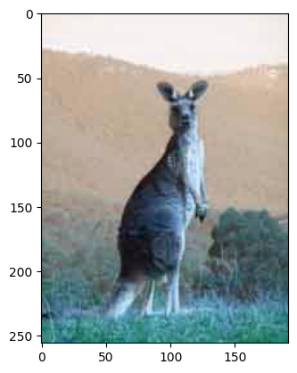
OpenCV uses BGR internally while most other libraries use RGB. This usually isn’t an issue unless you read an image with opencv and try to plot it with, say, matplotlib (note the flipped color channels in the image above). Then you’ll need to switch the channels around. Here is how to do that.
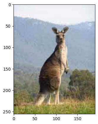
plt.imshow(img[:, :, ::-1]);
Time Test
%timeit cv2_img = cv2.imread(image_path)
487 µs ± 5 µs per loop (mean ± std. dev. of 7 runs, 1,000 loops each)
PIL
You can also use PIL for this.
from PIL import Image
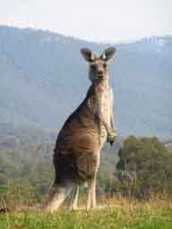
pil_img = Image.open(image_path) # This is already from an img
Note that PIL returns a special file type that you can display right away in a Jupyter Notebook.
pil_img
Time Test
%timeit pil_img = Image.open(image_path)
234 µs ± 4.71 µs per loop (mean ± std. dev. of 7 runs, 1,000 loops each)
PIL is incredibly fast at reading images.
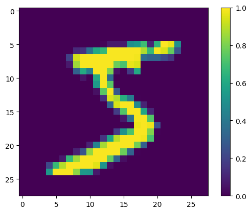
Visualizing from TensorFlow Datasets
import tensorflow as tf
(x_train, y_train), (x_test, y_test) = tf.keras.datasets.mnist.load_data()

x_train, x_test = x_train / 255.0, x_test / 255.0

print("Number of training examples:", len(x_train))
print("Number of test examples:", len(x_test))
Number of training examples: 60000
Number of test examples: 10000
print(y_train[0])

plt.imshow(x_train[0, :, :])
plt.colorbar();
5
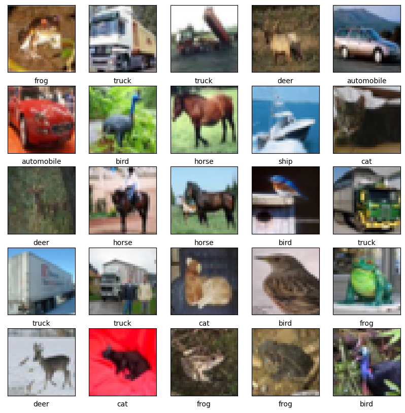
Plotting Multiple Images
Here’s an example of plotting multiple images with the label below it. It’s commonly done to visualize datasets.
import tensorflow as tf

from tensorflow.keras import datasets
import matplotlib.pyplot as plt
(train_images, train_labels), (test_images, test_labels) = datasets.cifar10.load_data()


train_images, test_images = train_images / 255.0, test_images / 255.0
class_names = ['airplane', 'automobile', 'bird', 'cat', 'deer',
               'dog', 'frog', 'horse', 'ship', 'truck']

plt.figure(figsize=(10,10))
for i in range(25):
    plt.subplot(5,5,i+1)
    plt.xticks([])
    plt.yticks([])
    plt.grid(False)
    plt.imshow(train_images[i], cmap=plt.cm.binary)
    plt.xlabel(class_names[train_labels[i][0]])
plt.show()