
Let’s look at how to explore images in Python. We’ll use the popular and active Pillow fork of PIL, the Python Imaging Library.
Table of Contents
from PIL import Image
import numpy as np
from matplotlib import pyplot as plt
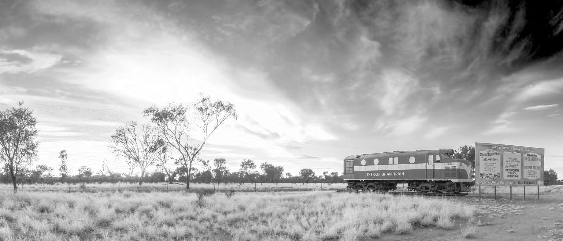
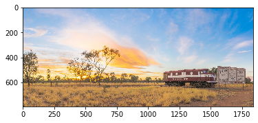
file_name = 'old_ghan.jpg'
im = Image.open(file_name)
im

Filtering by color
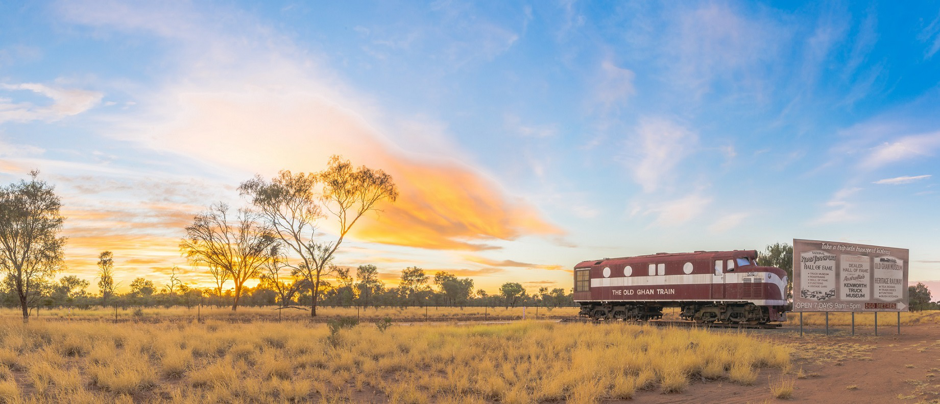
PIL reads in an image using three different color filters: red, green, and blue. In the picture above, the top right corner is mostly blue. Thus when we extract the colors, there should be very little red in that corner but lots of blue. So it will be dark in the red filter and light in the blue filter.
Let’s extract the colors individually and look at them.
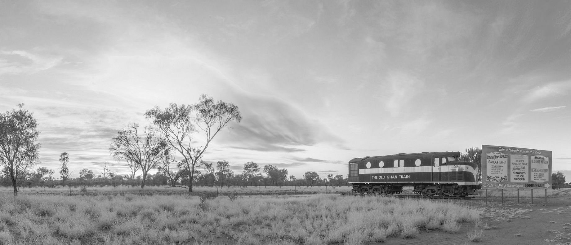
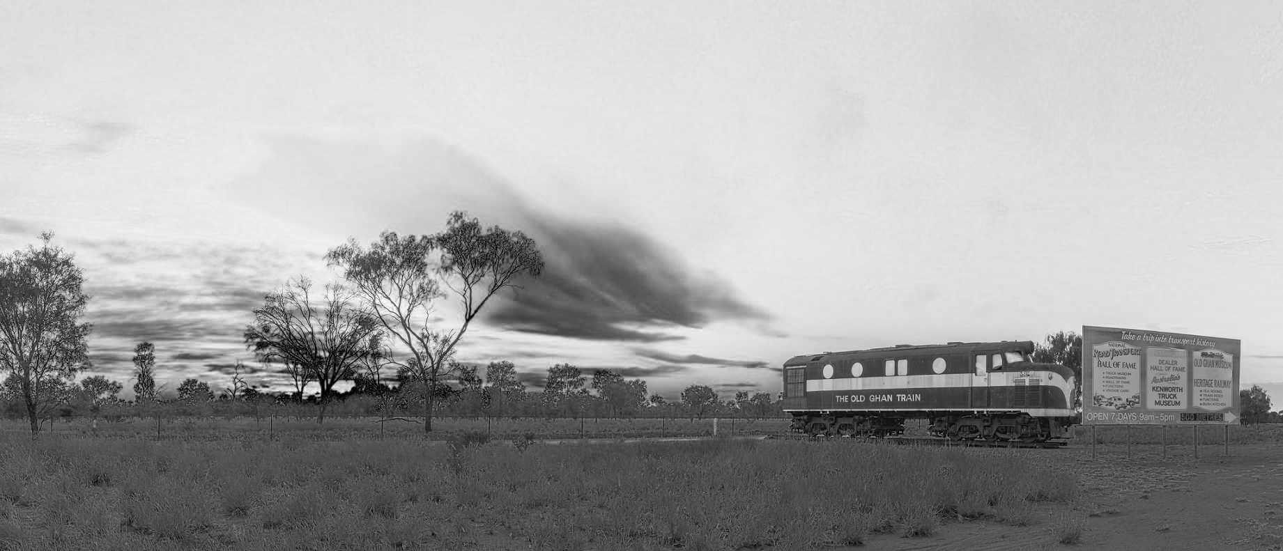
# Colors in the order of red, green, blue
r,g,b = im.split()
r
g
b
Converting to a matrix
A digital photograph is just a collection of numbers, and the great thing about a collection of numbers is that you can do data science with it. To do any data science on the images, we’ll need to look at them as n-dimensional arrays (ndarrays). This will allow us to apply all the linear algebra tools that are common in data science.
img_array = np.array(im)
print(img_array.shape)
(791, 1841, 3)
The array consists of three matrices, one each for red, green, and blue. Each individual matrix is the height by the width of the image.
Now let’s look at the top right corner of the image. For the red filter, it should all be low numbers, but for the blue filter it should be very high
def see_top_right_corner(array, layer, amount):
    single_color = array[:,:,layer]
    corner = single_color[0:amount, -amount-1:-1]
    return corner
Let’s look at the red filter (array 0)
see_top_right_corner(img_array, 0, 8)
array([[4, 3, 3, 1, 0, 0, 0, 0],
       [4, 3, 3, 1, 0, 0, 0, 0],
       [3, 3, 3, 1, 0, 0, 0, 0],
       [2, 2, 1, 1, 0, 0, 0, 0],
       [2, 2, 0, 1, 0, 0, 0, 0],
       [2, 2, 0, 0, 0, 0, 0, 0],
       [1, 0, 0, 0, 0, 0, 0, 0],
       [0, 0, 0, 0, 0, 0, 0, 0]], dtype=uint8)
The numbers are on a scale of 0-255, so these values are very low, indicating there’s not much red in the top right corner. Now let’s look at blue.
see_top_right_corner(img_array, 2, 8)
array([[215, 215, 217, 217, 217, 217, 217, 216],
       [215, 215, 217, 217, 217, 217, 217, 216],
       [215, 215, 217, 217, 217, 217, 217, 216],
       [214, 214, 217, 217, 217, 217, 217, 216],
       [214, 216, 216, 217, 217, 217, 217, 217],
       [214, 216, 216, 216, 217, 217, 217, 217],
       [213, 216, 216, 216, 216, 217, 217, 217],
       [215, 216, 216, 216, 216, 217, 217, 217]], dtype=uint8)
You can also visualize it after converting it to an ndarray. This means you can perform some operations on it and then see your results. You can do this with either PIL or Matplotlib.
# Using PIL.Image
Image.fromarray(img_array)
# Using matplotlib.pyplot
plt.imshow(img_array, interpolation='nearest')
plt.show()
Greyscale
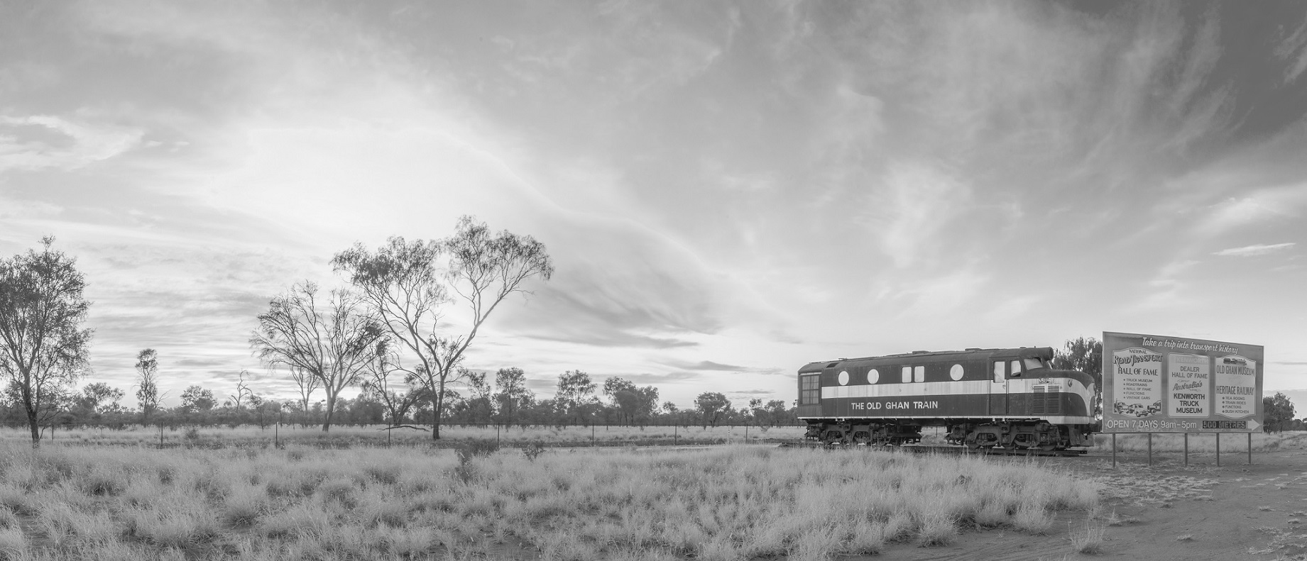
Although the individual filters are grey, using just one of them generally isn’t the best way to convert to greyscale. Pillow (and other image libraries, like OpenCV) has a way to combine the different individual colors into a greyscale that most closely matches what you would expect. In this case, you call the .convert("L") method. The “L” is for “luminosity” because we’re converting it to a single luminosity measure. You’ll also see .convert("LA"), which means luminosity and alpha (transparency).
im.convert("L")
Resizing
Pillow can also resize images. It’s recommended that you pass the Image.ANTIALIAS to the call.
# Preserve the original dimensions
h_over_w = im.size[1]/im.size[0]
new_width = 500
im_resize = im.resize((new_width, int(new_width*h_over_w)), Image.ANTIALIAS)
im_resize

Metadata
You can also look at metadata using Pillow.
im._getexif()
{296: 2,
 34665: 218,
 271: 'NIKON CORPORATION',
 272: 'NIKON D7200',
 305: 'Adobe Photoshop Lightroom 6.12 (Windows)',
 306: '2017:10:16 13:48:45',
 282: 240.0,
 283: 240.0,
 36864: b'0230',
 37377: 3.0,
 37378: 8.918863,
 36867: '2017:03:31 06:41:30',
 36868: '2017:03:31 06:41:30',
 37380: -2.0,
 37381: 1.0,
 37383: 5,
 37384: 0,
 37385: 16,
 37386: 24.0,
 40961: 1,
 41987: 0,
 41988: 1.0,
 41486: 2558.6412048339844,
 41487: 2558.6412048339844,
 41488: 3,
 37521: '0411',
 37522: '0411',
 41994: 0,
 41996: 0,
 41495: 2,
 41728: b'\x03',
 33434: 0.125,
 33437: 22.0,
 41729: b'\x01',
 34850: 1,
 41730: b'\x02\x00\x02\x00\x00\x01\x01\x02',
 41985: 0,
 34855: 100,
 41986: 1,
 34864: 2,
 42033: '2529332',
 42034: (24.0, 24.0, 1.4, 1.4),
 42036: '24.0 mm f/1.4',
 41989: 36,
 41990: 0,
 41991: 0,
 41992: 0,
 41993: 0}
It’s not particularly intuitive. For example, the creation date is number 36867. To see the meanings of these values, see the bottom of this webpage by Nicholas Armstrong.
im._getexif()[36867]
'2017:03:31 06:41:30'