
This post is in a series on machine learning with unbalanced datasets. This post focuses on the training aspect. For background, please see the setup post.
When we think about training a machine learning model on an unbalanced dataset, we need to answer several questions along the way. The first is, given that our population is unbalanced, should our training data be unbalanced as well? Or is it better to have balanced training data? And, if we want to balance the data, what’s the best way to do it?
Adding more data to the less common class is almost certainly the best approach. But if that’s not possible, what can we do? The two most popular methods for rebalancing data are adding more weight to the less common class or oversampling it. Which is better?
Table of Contents
- Experiment #1 - Should the Training Data Be Balanced or Unbalanced?
- Experiment #2 - Using class_weight
- Experiment #2b - More class_weight
- Experiment #3 Using Oversampling
- Conclusion
%run 2021-05-01-experiments-on-unbalanced-datasets-setup.ipynb
Classes:
 ['cats', 'dogs']
There are a total of 5000 cat images in the entire dataset.
There are a total of 5000 dog images in the entire dataset.
Experiment #1 - Should the Training Data Be Balanced or Unbalanced?
For our first experiment we’ll make a couple train datasets. One option is to have a balanced dataset, the other is to allow it to be unbalanced to match the “real world”. Let’s see which one produces better results. The validation and test sets will be unbalanced to match the real world distribution.
cat_list_train_balanced, cat_list_train_unbalanced, cat_list_val, cat_list_test = subset_dataset(cat_list_ds, [1500, 1500, 1000, 1000])
dog_list_train_balanced, dog_list_train_unbalanced, dog_list_val, dog_list_test = subset_dataset(dog_list_ds, [1500, 150, 100, 100])
train_ds_balanced = prepare_dataset(cat_list_train_balanced, dog_list_train_balanced)
train_ds_unbalanced = prepare_dataset(cat_list_train_unbalanced, dog_list_train_unbalanced)
val_ds = prepare_dataset(cat_list_val, dog_list_val)
test_ds = prepare_dataset(cat_list_test, dog_list_test)
Now let’s train the models. We’re going to train 10 models and take the average of the metrics to reduce the noise.
history_balanced, preds_balanced, evals_balanced = run_experiment(train_ds_balanced, val_ds, test_ds)
69/69 [==============================] - 10s 141ms/step
69/69 [==============================] - 10s 138ms/step
69/69 [==============================] - 10s 139ms/step
69/69 [==============================] - 10s 141ms/step
69/69 [==============================] - 10s 139ms/step
69/69 [==============================] - 10s 139ms/step
69/69 [==============================] - 10s 140ms/step
69/69 [==============================] - 10s 140ms/step
69/69 [==============================] - 10s 139ms/step
69/69 [==============================] - 10s 140ms/step
history_unbalanced, preds_unbalanced, evals_unbalanced = run_experiment(train_ds_unbalanced, val_ds, test_ds)
69/69 [==============================] - 10s 138ms/step
69/69 [==============================] - 10s 138ms/step
69/69 [==============================] - 10s 139ms/step
69/69 [==============================] - 10s 138ms/step
69/69 [==============================] - 10s 138ms/step
69/69 [==============================] - 10s 138ms/step
69/69 [==============================] - 10s 138ms/step
69/69 [==============================] - 10s 139ms/step
69/69 [==============================] - 10s 138ms/step
69/69 [==============================] - 10s 138ms/step
Experiment #1 Evaluation
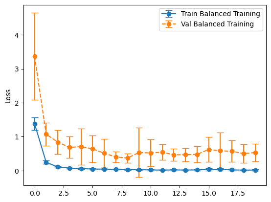
plot_losses(history_balanced, "Balanced Training")
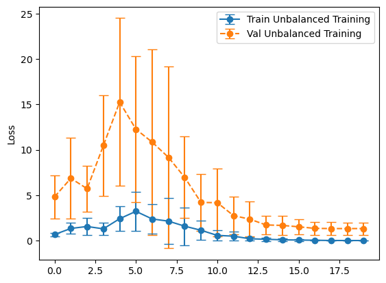
plot_losses(history_unbalanced, "Unbalanced Training")
Now let’s look at the metrics and results.
balanced_mean_metrics = get_means(evals_balanced)
unbalanced_mean_metrics = get_means(evals_unbalanced)
for name, value in zip(metric_names, balanced_mean_metrics):
    print(f"{name}: {value}")
loss: 0.4516646429896355
tp: 93.5
fp: 56.9
tn: 943.1
fn: 6.5
accuracy: 0.9423636257648468
precision: 0.6367852687835693
recall: 0.9350000023841858
for name, value in zip(metric_names, unbalanced_mean_metrics):
    print(f"{name}: {value}")
loss: 0.7680775374174118
tp: 71.9
fp: 4.5
tn: 995.5
fn: 28.1
accuracy: 0.9703636467456818
precision: 0.9419323027133941
recall: 0.7189999997615815
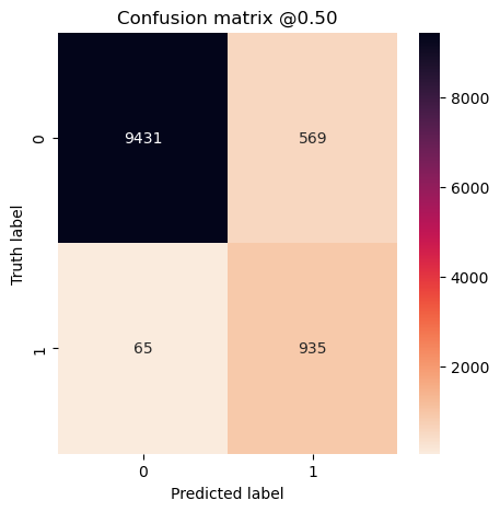
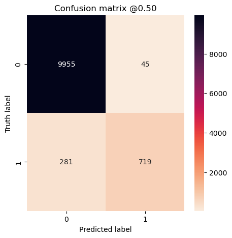
The model trained on the unbalanced dataset has a higher accuracy, but it has lower recall, meaning it misses more of the minority class (dogs).
To make a confusion matrix I’ll simply concatenate all the results together.
concat_preds_balanced = np.concatenate(preds_balanced)
concat_preds_unbalanced = np.concatenate(preds_unbalanced)
true_labels = tf.concat([y for x, y in test_ds], axis=0)
num_runs = len(preds_balanced)
concat_labels = np.tile(true_labels.numpy(), num_runs)
plot_cm(concat_labels, concat_preds_balanced)
plot_cm(concat_labels, concat_preds_unbalanced)
Experiment #2 - Using class_weight
We know from the above experiments that training on balanced data is better than training on unbalanced, but what if we can’t get balanced data? There are many ways to try to get around this. One of the most popular is by adjusting the weights of the less common class so the model learns more from them. We know we have 10 times as many cats as dogs, so we’ll weigh the dogs 10 times as much.
class_weight = {0:1, 1:10}
history_weighted, preds_weighted, evals_weighted = run_experiment(
    train_ds_unbalanced, val_ds, test_ds, class_weight=class_weight
)
69/69 [==============================] - 10s 139ms/step
69/69 [==============================] - 10s 138ms/step
69/69 [==============================] - 10s 138ms/step
69/69 [==============================] - 10s 139ms/step
69/69 [==============================] - 10s 137ms/step
69/69 [==============================] - 11s 137ms/step
69/69 [==============================] - 10s 138ms/step
69/69 [==============================] - 10s 137ms/step
69/69 [==============================] - 10s 139ms/step
69/69 [==============================] - 10s 137ms/step
Experiment #2 Evaluation
eval_weighted_means = get_means(evals_weighted)
for name, value in zip(metric_names, eval_weighted_means):
    print(f"{name}: {value}")
loss: 0.7273299664258956
tp: 77.5
fp: 4.8
tn: 995.2
fn: 22.5
accuracy: 0.9751818418502808
precision: 0.9419276118278503
recall: 0.774999988079071
concat_preds = np.concatenate(preds_weighted)
plot_cm(concat_labels, concat_preds)

Interestingly, if you undo the difference in the unbalanced data by adjusting the weights, it goes too far. But not always…
Experiment #2b - More class_weight
class_weight2 = {0:1, 1:25}
history_weighted2, preds_weighted2, evals_weighted2 = run_experiment(
    train_ds_unbalanced, val_ds, test_ds, class_weight=class_weight2
)
69/69 [==============================] - 10s 137ms/step
69/69 [==============================] - 10s 137ms/step
69/69 [==============================] - 11s 137ms/step
69/69 [==============================] - 10s 138ms/step
69/69 [==============================] - 10s 138ms/step
69/69 [==============================] - 10s 138ms/step
69/69 [==============================] - 10s 136ms/step
69/69 [==============================] - 10s 138ms/step
69/69 [==============================] - 10s 137ms/step
69/69 [==============================] - 10s 138ms/step
Experiment #2b Evaluation
eval_weighted_means2 = get_means(evals_weighted2)
for name, value in zip(metric_names, eval_weighted_means2):
    print(f"{name}: {value}")
loss: 1.357473886013031
tp: 75.5
fp: 6.1
tn: 993.9
fn: 24.5
accuracy: 0.9721818387508392
precision: 0.9258232951164246
recall: 0.7550000011920929
concat_preds2 = np.concatenate(preds_weighted2)
plot_cm(concat_labels, concat_preds2)

This definitely got more of the dog images. Using class_weight can be very helpful when trying to find a high recall, low precision model. This could be useful for something like frontline cancer detection where you want to tell people that they don’t have cancer and be right a very high percentage of the time, or tell people that they might and further testing is needed. However, I find the results using class_weight inconsistent and can make the model performance swing wildly from high precision to low precision, so it’s not my preferred approach.
Experiment #3 Using Oversampling
I generally prefer oversampling. Here’s how to do it with tf.data datasets. We know it’s a 10:1 ratio, so we have to repeat the dogs 10 times.
resampled_ds = tf.data.experimental.sample_from_datasets(
    [cat_list_train_unbalanced, dog_list_train_unbalanced.repeat(10)], weights=[0.5, 0.5], seed=42
)
resampled_ds = resampled_ds.map(parse_file)
resampled_ds = resampled_ds.batch(BATCH_SIZE).prefetch(AUTOTUNE)
Just to make sure it’s what we want we can take a look at the labels.
resampled_true_labels = tf.concat([y for x, y in resampled_ds], axis=0)
resampled_true_labels
<tf.Tensor: shape=(3000,), dtype=int64, numpy=array([1, 1, 1, ..., 1, 1, 1])>
sum(resampled_true_labels)
<tf.Tensor: shape=(), dtype=int64, numpy=1500>
The sum is half the total, so half are 1 and half are 0, which is what we expected. Let’s train some models.
history_oversampled, preds_oversampled, evals_oversampled = run_experiment(resampled_ds, val_ds, test_ds)
69/69 [==============================] - 10s 137ms/step
69/69 [==============================] - 10s 137ms/step
69/69 [==============================] - 10s 137ms/step
69/69 [==============================] - 10s 137ms/step
69/69 [==============================] - 10s 138ms/step
69/69 [==============================] - 10s 137ms/step
69/69 [==============================] - 10s 138ms/step
69/69 [==============================] - 10s 138ms/step
69/69 [==============================] - 10s 138ms/step
69/69 [==============================] - 10s 137ms/step
Experiment #3 Evaluation
eval_oversampled_means = get_means(evals_oversampled)
for name, value in zip(metric_names, eval_oversampled_means):
    print(f"{name}: {value}")
loss: 0.6174567520618439
tp: 76.6
fp: 6.4
tn: 993.6
fn: 23.4
accuracy: 0.9729091167449951
precision: 0.9241096913814545
recall: 0.7660000026226044
concat_preds_oversampled = np.concatenate(preds_oversampled)
plot_cm(concat_labels, concat_preds_oversampled)

So even though it’s not perfect, we got a decent result. This does cause a problem though because we’ve overfit the less common class and not the other class. Depending on how much data we have, we could add undersampling as well. In general I would prefer not to undersample but instead to add data augmentation instead.
Conclusion
You’ll notice that no result was always better than the other results. It depended on the exact parameters and what metrics are most important. If you only care about recall, you may want to weigh the target labels extra heavily. You can also combine class_weight and oversampling and tweak both to your liking.