
The Jupyter Notebook is a great tool for writing and exploring code as well as prototyping ideas. It’s one of my favorite ways to write code, in part because of all the great features it has. This post demonstrates some of my favorite features.
Table of Contents
- Jupyter Notebook extensions
- Shell Commands
- Magic Commands
- Debugging
- Getting Help and Viewing Source Code
- Widgets
- Converting to other formats with nbconvert
- Little Tricks
- Viewer
- Examples
- Version Control
Jupyter Notebook extensions
One of the many great things about Jupyter Notebooks is the ability to add extensions.
Installation
The easiest way to add Jupyter Notebook extensions is through nbextensions. You can install it using conda-forge:
conda install -c conda-forge jupyter_contrib_nbextensions
You can also use pip:
pip install jupyter_contrib_nbextensions
Then:
- Enter:
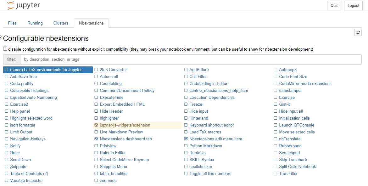
jupyter contrib nbextension install --user - Open up Jupyter Notebook and you will have a tab called Nbextensions. You can enable individual extensions from this tab.
Formatting Extensions
Autopep8
You can use Autopep8 to format your code to be consistent with the PEP8 style guide.
Install with pip install autopep8, then enable it.
Jupyter Black
Jupyter Black brings the black formatter to Python.
- Install it with:
jupyter nbextension install https://github.com/drillan/jupyter-black/archive/master.zip --sys-prefix. - Enable it in the Nbextensions tab:

I like to customize the black formatter by changing the line length. To do this, you will have to select Jupyter Black in the Nbextensions tab as shown above and scroll down until you see the image below. You can add the line_length as an argument to black.FileMode() as shown in the red circle below:

spellchecker
spellchecker does exactly what you think it does.
Hinterland
Adds autocompletion to Jupyter Notebooks, which normally requires hitting the Tab button.
table_beautifier
Adds bootstrap style to tables, which is great because it makes pandas DataFrames sortable by default.
Other Tools (Evaluating)
Beautiful LaTeX
Check out handcalcs if you want to automatically create beautiful LaTeX equations.
Shell Commands
You can also use shell commands inside Jupyter Notebooks.
Built-in
Some are built-in so you can type them directly, such as ls or pwd.
pwd
'C:\\Users\\Julius\\Google Drive\\JupyterNotebooks\\Blog'
Other (such as pip)
To access other shell commands, you will need to prefix them with a !. For example, you can pip install directly from Jupyter Notebooks:
!pip install numpy
Magic Commands
Jupyter Notebooks have another type of command known as magic commands. You can view all the magic commands by entering %quickref into your notebook, but here are some of my favorites:
Display all your global variables with %whos
It’s easy to lose track of your global variables, especially if you run your cells out of order. Fortunately, you can use the magic command %whos to display them all.

Sharing Values with %store
You can use magic commands to store values in one notebook and load them in another. Here’s an example:
x = 5
Now you save it like so:
%store x
Stored 'x' (int)
And you can load it:
%store -r x
Running files with %run
You can use %run my_file.py to run a separate file. You can also do this with other Jupyter Notebooks by doing %run my_notebook.ipynb.
Measuring Execution Time
You can use timeit to see how long it takes your code to run. To measure a single line of code, you can use %timeit:
%timeit [x**2 for x in range(1000)]
To measure multiple lines of code, use %%timeit at the beginning of a cell:
%%timeit
squares = []
for x in range(1000):
    squares.append(x**2)
Debugging
Jupyter Notebooks have an amazing command for debugging. If you are running code and get an error, even if it’s deep inside a function, you can type %debug into a cell and it will open up ipdb at the exact location the error occurred with all the values as they were. It’s amazing. Here’s an example:
def foo():
    soln = 'a' + 1
    return soln
foo()
---------------------------------------------------------------------------

TypeError                                 Traceback (most recent call last)

<ipython-input-4-c19b6d9633cf> in <module>
----> 1 foo()


<ipython-input-3-84285e1acb14> in foo()
      1 def foo():
----> 2     soln = 'a' + 1
      3     return soln


TypeError: can only concatenate str (not "int") to str
%debug
> [1;32m<ipython-input-3-84285e1acb14>[0m(2)[0;36mfoo[1;34m()[0m
[1;32m 1 [1;33m[1;32mdef[0m [0mfoo[0m[1;33m([0m[1;33m)[0m[1;33m:[0m[1;33m[0m[1;33m[0m[0m
[0m[1;32m----> 2 [1;33m [0msoln[0m [1;33m=[0m [1;34m'a'[0m [1;33m+[0m [1;36m1[0m[1;33m[0m[1;33m[0m[0m
[0m[1;32m 3 [1;33m [1;32mreturn[0m [0msoln[0m[1;33m[0m[1;33m[0m[0m
[0m
ipdb> exit
Getting Help and Viewing Source Code
Jupyter Notebooks have a lot of support for looking into code right from the notebook. Here are some examples.
Command Palette
Jupyter Notebooks has a command palette that you can access with Ctrl + Shift + P (Windows/Linux) / Cmd + Shift + P (Mac) (just like VSCode). From there you can search for whatever feature you’re looking for.
Shift + Tab
Shift + Tab is a great keyboard shortcut that every Jupyter Notebook user should know. You simply start to call a function and when you’re inside the parentheses and can’t remember the right inputs, hit Shift + Tab and it will show you the documentation. If you hit Tab multiple times while holding Shift it cycles through various displays of the documentation. Try it out!
Question Marks
You can put a question mark behind any function or class to pull up the docstring. It creates a pop-up from the bottom of the screen, so you won’t be able to see it in this post, but here’s an example.
def func_with_docstring():
    """
    This is a useful docstring
    """
    return 1
func_with_docstring?
Even better than that, just put two question marks behind something to view the source code.
func_with_docstring??
This shows you the docstring as before but then the entire code. Amazing!
Also If you just wanted to see the docstring, you could call help. This prints the docstring, so you’ll be able to see it in this case.
help(func_with_docstring)
Help on function func_with_docstring in module __main__:

func_with_docstring()
    This is a useful docstring
Widgets
You can build beautiful and functional widgets right into your notebooks with ipywidgets. This is such a great tool to really add some power to your notebooks.
Converting to other formats with nbconvert
Convert Jupyter Notebooks to various formats, including HTML, LaTeX, PDF, and Markdown
jupyter nbconvert --to html mynotebook.ipynb
or
jupyter nbconvert --to markdown mynotebook.ipynb
See how I use it to prepare Jupyter Notebooks for my blog.
If you want to publish the notebook without code, you can also do this:
jupyter nbconvert --to markdown --no-input mynotebook.ipynb
Little Tricks
Splitting Cells
One hot key that I like but sometimes forget is how to split a cell where my cursor is. So I just open up the command palette and type in “split” and I see that it is Ctrl + Shift + - (Windows/Linux/Mac).
Printing LaTeX
Jupyter Notebooks use MathJax to render LaTeX in Markdown. To add LaTeX, simply surround your statement with $$:
Some things that work in Jupyter Notebooks don’t work with the renderer I use for this blog, so I can’t show everything. But in Jupyter Notebooks you can use LaTeX with a single $ and use a double $$ to center the expression.
Suppressing Output
When you run a command in Jupyter Notebooks the last output is printed. But if for some reason you don’t want this, you can always suppress it with a semicolon. For example, you often don’t want to return from matplotlib commands, so you can:
plt.show();
Viewer
There’s a really simple way to share beautiful notebooks, and it’s called nbviewer
Examples
There are so many awesome examples of Jupyter Notebooks out there. Here are some great ones:
A gallery of interesting Jupyter Notebooks
Version Control
By default, version control doesn’t work that well with Jupyter Notebooks. But there are tools to help. For open source work and commercial work if you want to pay for it, there is ReviewNB. If you want to use a tool that is free and open source, I recommend nbdime, which is what I use. Here are some example commands:
Traditionally with git, you can compare your changes with the previous commit with git diff HEAD^ HEAD. With nbdime, you can do nbdiff-web HEAD^ HEAD to see a visual of the differences.