
It’s important to know whether a model has been trained well or not. One way to do this is to look at the model weights. But it’s hard to know what exactly they’re telling you - you need something to compare the weights to. In this post, I’m going to look at the weight statistics for a couple of well-trained networks, which can be used as comparison points.
We’ll use well-known pre-trained models like VGG-16 and ResNet50. But before we do that, let’s look at an untrained network so we can see how the weights change after they are trained. We’ll see how the distribution changes from an untrained network to a trained one.
Table of Contents
import tensorflow as tf
import math
from tensorflow.keras.applications import ResNet50, VGG16
import numpy as np
from matplotlib import pyplot as plt
We’re going to use models that are provided in keras. These are easy to work with and support random initialization, ImageNet weights, and loading custom weights. To start with, we’ll use random weights. Let’s download our model.
Untrained VGG-16
vgg_model_untrained = VGG16(weights=None)
Let’s look at the model architecture.
vgg_model_untrained.summary()
Model: "vgg16"
_________________________________________________________________
Layer (type)                 Output Shape              Param #
=================================================================
input_1 (InputLayer)         [(None, 224, 224, 3)]     0
_________________________________________________________________
block1_conv1 (Conv2D)        (None, 224, 224, 64)      1792
_________________________________________________________________
block1_conv2 (Conv2D)        (None, 224, 224, 64)      36928
_________________________________________________________________
block1_pool (MaxPooling2D)   (None, 112, 112, 64)      0
_________________________________________________________________
block2_conv1 (Conv2D)        (None, 112, 112, 128)     73856
_________________________________________________________________
block2_conv2 (Conv2D)        (None, 112, 112, 128)     147584
_________________________________________________________________
block2_pool (MaxPooling2D)   (None, 56, 56, 128)       0
_________________________________________________________________
block3_conv1 (Conv2D)        (None, 56, 56, 256)       295168
_________________________________________________________________
block3_conv2 (Conv2D)        (None, 56, 56, 256)       590080
_________________________________________________________________
block3_conv3 (Conv2D)        (None, 56, 56, 256)       590080
_________________________________________________________________
block3_pool (MaxPooling2D)   (None, 28, 28, 256)       0
_________________________________________________________________
block4_conv1 (Conv2D)        (None, 28, 28, 512)       1180160
_________________________________________________________________
block4_conv2 (Conv2D)        (None, 28, 28, 512)       2359808
_________________________________________________________________
block4_conv3 (Conv2D)        (None, 28, 28, 512)       2359808
_________________________________________________________________
block4_pool (MaxPooling2D)   (None, 14, 14, 512)       0
_________________________________________________________________
block5_conv1 (Conv2D)        (None, 14, 14, 512)       2359808
_________________________________________________________________
block5_conv2 (Conv2D)        (None, 14, 14, 512)       2359808
_________________________________________________________________
block5_conv3 (Conv2D)        (None, 14, 14, 512)       2359808
_________________________________________________________________
block5_pool (MaxPooling2D)   (None, 7, 7, 512)         0
_________________________________________________________________
flatten (Flatten)            (None, 25088)             0
_________________________________________________________________
fc1 (Dense)                  (None, 4096)              102764544
_________________________________________________________________
fc2 (Dense)                  (None, 4096)              16781312
_________________________________________________________________
predictions (Dense)          (None, 1000)              4097000
=================================================================
Total params: 138,357,544
Trainable params: 138,357,544
Non-trainable params: 0
_________________________________________________________________
We’ll look at the first and last convolution and dense (aka fully connected) layers and see how they change and why. We can get a list of all the layers by calling .layers like so:
vgg_model_untrained.layers
[<tensorflow.python.keras.engine.input_layer.InputLayer at 0x16c4df909c8>,
 <tensorflow.python.keras.layers.convolutional.Conv2D at 0x16c43ddbe88>,
 <tensorflow.python.keras.layers.convolutional.Conv2D at 0x16c4e8f7b48>,
 <tensorflow.python.keras.layers.pooling.MaxPooling2D at 0x16c4eaeaf88>,
 <tensorflow.python.keras.layers.convolutional.Conv2D at 0x16c4eaec408>,
 <tensorflow.python.keras.layers.convolutional.Conv2D at 0x16c4eb06b88>,
 <tensorflow.python.keras.layers.pooling.MaxPooling2D at 0x16c4eb0be88>,
 <tensorflow.python.keras.layers.convolutional.Conv2D at 0x16c4eb12508>,
 <tensorflow.python.keras.layers.convolutional.Conv2D at 0x16c4eb22988>,
 <tensorflow.python.keras.layers.convolutional.Conv2D at 0x16c4eb24648>,
 <tensorflow.python.keras.layers.pooling.MaxPooling2D at 0x16c4eb2fe08>,
 <tensorflow.python.keras.layers.convolutional.Conv2D at 0x16c4eb36e88>,
 <tensorflow.python.keras.layers.convolutional.Conv2D at 0x16c4eb446c8>,
 <tensorflow.python.keras.layers.convolutional.Conv2D at 0x16c4eb48588>,
 <tensorflow.python.keras.layers.pooling.MaxPooling2D at 0x16c4eb53a88>,
 <tensorflow.python.keras.layers.convolutional.Conv2D at 0x16c4eb55c48>,
 <tensorflow.python.keras.layers.convolutional.Conv2D at 0x16c4ecb1cc8>,
 <tensorflow.python.keras.layers.convolutional.Conv2D at 0x16c4ecbbc08>,
 <tensorflow.python.keras.layers.pooling.MaxPooling2D at 0x16c4ecc4c48>,
 <tensorflow.python.keras.layers.core.Flatten at 0x16c4eccc908>,
 <tensorflow.python.keras.layers.core.Dense at 0x16c4e8d9a88>,
 <tensorflow.python.keras.layers.core.Dense at 0x16c4ecd3b48>,
 <tensorflow.python.keras.layers.core.Dense at 0x16c4ecdea08>]
Now let’s extract the weights.
first_vgg_conv_weights_untrained, first_vgg_conv_biases_untrained = vgg_model_untrained.layers[1].get_weights()
last_vgg_conv_weights_untrained, last_vgg_conv_biases_untrained = vgg_model_untrained.layers[-6].get_weights()
first_vgg_fc_weights_untrained, first_vgg_fc_biases_untrained = vgg_model_untrained.layers[-3].get_weights()
last_vgg_fc_weights_untrained, last_vgg_fc_biases_untrained = vgg_model_untrained.layers[-1].get_weights()
Untrained VGG-16 Convolutional Layers
We’ll create a simple function to show summary statistics and plot a histogram.
def print_stats(nparray):
    print("Shape: ", nparray.shape)
    print("Mean: ", np.mean(nparray))
    print("Standard Deviation: ", np.std(nparray))
    print("Variance: ", np.var(nparray))
    print("Min: ", np.min(nparray))
    print("Max: ", np.max(nparray))
def plot_histo(nparray, model_name, layer, param):
    assert param in {'weights', 'biases'}
    plt.figure(figsize=(8, 6))
    plt.hist(np.asarray(nparray).flatten(), rwidth=0.9)
    plt.title(f"Plot of {model_name} {param} in {layer} layer")
    plt.xlabel("Value")
    plt.ylabel("Count")
def summarize(nparray, model_name=None, layer=None, param=None):
    print_stats(nparray)
    plot_histo(nparray, model_name, layer, param)
Let’s look at our first weights and biases
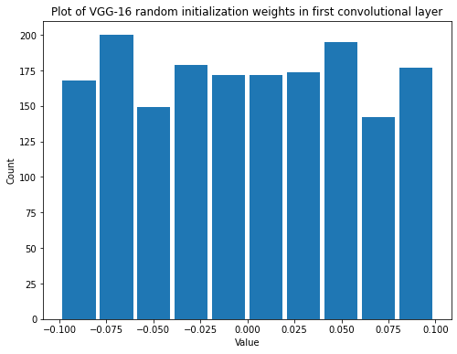
summarize(first_vgg_conv_weights_untrained, 'VGG-16 random initialization', 'first convolutional', 'weights')
Shape:  (3, 3, 3, 64)
Mean:  -2.0897362e-05
Standard Deviation:  0.057159748
Variance:  0.003267237
Min:  -0.09954555
Max:  0.09961195
print_stats(first_vgg_conv_biases_untrained)
Shape:  (64,)
Mean:  0.0
Standard Deviation:  0.0
Variance:  0.0
Min:  0.0
Max:  0.0
The first thing we see is that the weights and biases are initialized differently. Specifically, the weights are initialized to some distribution of random values and the biases are all initialized to 0.
But what is the distribution that the weights are initialized to? For a convolutional layer, the weights are initialized to glorot_uniform. This is the initialization method described in Understanding the difficulty of training deep feedforward neural networks by Xavier Glorot and Yoshua Bengio. In TensorFlow it’s called “Glorot initialization”, but I see it more commonly referred to as “Xavier initialization”.
We can confirm that this is what TensorFlow is doing by calling this method directly and seeing that it is the same.
initializer = tf.keras.initializers.GlorotUniform()
values = initializer(shape=(3, 3, 3, 64))
print_stats(values)
Shape:  (3, 3, 3, 64)
Mean:  0.00015374094
Standard Deviation:  0.056950122
Variance:  0.0032433164
Min:  -0.09963174
Max:  0.09960838
Let’s step through this process. The idea is to make the weights uniformly distributed between positive and negative \(\frac{\sqrt{6}}{\sqrt{fan_{in} + fan_{out}}}\)
fan_in is the number of input connections and fan_out is the number of output connections. So for fan_in that’s the kernel size (3*3) times the number of input channels, which is 3. For fan_out, it’s the kernel size times the number of output channels, which is 64.
fan_in = 3*3*3
fan_out = 3*3*64
The variance, or scale as it is written in TensorFlow, is the inverse of the mean of those two.
scale = 1 / ((fan_in + fan_out) / 2.)
scale
0.003316749585406302
From there we can calculate the limit.
limit = math.sqrt(3.0 * scale)
limit
0.09975093361076329
Note what we’ve done is exactly the same as the original paper, the order is just a little bit different.

OK, now let’s look at the next layer. We know the bias is going to be zero but we can look at the weights.
summarize(last_vgg_conv_weights_untrained, 'VGG-16 random initialization', 'last convolutional', 'weights')
Shape:  (3, 3, 512, 512)
Mean:  -1.52503735e-05
Standard Deviation:  0.0147314165
Variance:  0.00021701462
Min:  -0.025515513
Max:  0.025515452
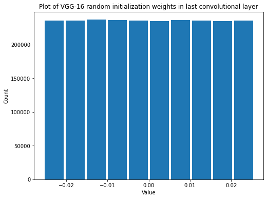
Now that there are so many values it’s much easier to see that it’s a uniform distribution. Also notice that the variance is much lower now. That’s because there are many more connections coming into and going out of the layer. We can calculate the variance and limit as we did before.
fan_in = 3*3*512
fan_out = 3*3*512
scale = 1 / ((fan_in + fan_out) / 2.)
scale
0.00021701388888888888
limit = math.sqrt(3.0 * scale)
limit
0.02551551815399144
And again we get the same values. Let’s look at them again.
initializer = tf.keras.initializers.GlorotUniform()
values = initializer(shape=(3, 3, 512, 512))
print_stats(values)
Shape:  (3, 3, 512, 512)
Mean:  -1.0009625e-05
Standard Deviation:  0.014722626
Variance:  0.00021675571
Min:  -0.025515513
Max:  0.0255155
Untrained VGG-16 Fully Connected Layers
Now let’s look at the fully connected layers. In the TensorFlow code for fully connected layers, you’ll also see that they use Xavier initialization. The first fully connected layer should have the lowest variance of all because it has the most connections.
print_stats(first_vgg_fc_weights_untrained)
Shape:  (25088, 4096)
Mean:  1.5987824e-06
Standard Deviation:  0.008278468
Variance:  6.853302e-05
Min:  -0.014338483
Max:  0.014338479
print_stats(first_vgg_fc_biases_untrained)
Shape:  (4096,)
Mean:  0.0
Standard Deviation:  0.0
Variance:  0.0
Min:  0.0
Max:  0.0
We see that the biases are still initialized to zero for the fully connected layers.
Now let’s look at the last layer.
print_stats(last_vgg_fc_weights_untrained)
Shape:  (4096, 1000)
Mean:  -3.772734e-06
Standard Deviation:  0.019808477
Variance:  0.00039237578
Min:  -0.034313176
Max:  0.03431317
The variance has increased compared with the first fully connected layer, as we expected.
Pre-trained VGG-16
vgg_model = VGG16(weights='imagenet')
first_vgg_conv_weights, first_vgg_conv_biases = vgg_model.layers[1].get_weights()
last_vgg_conv_weights, last_vgg_conv_biases = vgg_model.layers[-6].get_weights()
first_vgg_fc_weights, first_vgg_fc_biases = vgg_model.layers[-3].get_weights()
last_vgg_fc_weights, last_vgg_fc_biases = vgg_model.layers[-1].get_weights()
Pre-trained VGG-16 Convolutional Layers
summarize(first_vgg_conv_weights, 'VGG-16', 'first convolutional', 'weights')
Shape:  (3, 3, 3, 64)
Mean:  -0.0024379087
Standard Deviation:  0.20669945
Variance:  0.04272466
Min:  -0.67140007
Max:  0.6085159
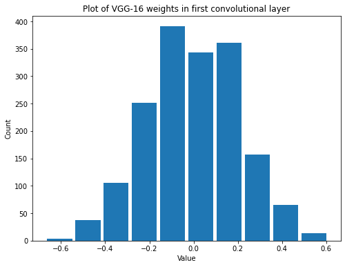
Looks like by the time the model is done training it ends up with closer to a uniform distribution.
And now the biases.
summarize(first_vgg_conv_biases, 'VGG-16', 'first convolutional', 'biases')
Shape:  (64,)
Mean:  0.5013912
Standard Deviation:  0.32847992
Variance:  0.10789906
Min:  -0.015828926
Max:  2.064037
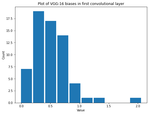
Now they’ve both changed but note that the distributions for the weights and biases are different. The weights are even centered around a mean of around 0 while the biases have a mean around 0.5 and range from 0 to 2.
If we compare them to the untrained weights, we see that the mean has stayed close to 0, but the variance and range have increased substantially.
Now let’s look at the last layers.
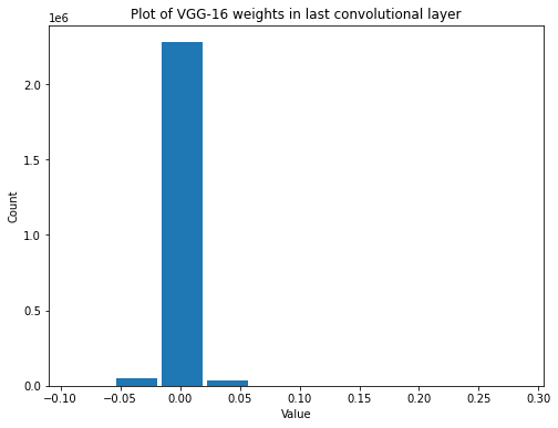
summarize(last_vgg_conv_weights, 'VGG-16', 'last convolutional', 'weights')
Shape:  (3, 3, 512, 512)
Mean:  -0.0010818949
Standard Deviation:  0.008478405
Variance:  7.1883354e-05
Min:  -0.09288482
Max:  0.28699666
summarize(last_vgg_conv_biases, 'VGG-16', 'last convolutional', 'biases')
Shape:  (512,)
Mean:  0.14986369
Standard Deviation:  0.4928213
Variance:  0.24287283
Min:  -0.50036746
Max:  9.431553

It’s interesting… It looks like the variance of the weights in convolutional layers decrease as we go deeper into the network. They all get closer and closer to zero. Let’s see if we can visualize that.
First we’ll extract all the convolutional layers.
vgg_conv_layers = [layer for layer in vgg_model.layers if isinstance(layer, tf.keras.layers.Conv2D)]
vgg_conv_layers
[<tensorflow.python.keras.layers.convolutional.Conv2D at 0x16c4f0fd708>,
 <tensorflow.python.keras.layers.convolutional.Conv2D at 0x16c4f2e4fc8>,
 <tensorflow.python.keras.layers.convolutional.Conv2D at 0x16c4f2d1508>,
 <tensorflow.python.keras.layers.convolutional.Conv2D at 0x16c4f2fad08>,
 <tensorflow.python.keras.layers.convolutional.Conv2D at 0x16c4f306888>,
 <tensorflow.python.keras.layers.convolutional.Conv2D at 0x16c4f30fec8>,
 <tensorflow.python.keras.layers.convolutional.Conv2D at 0x16c4f443288>,
 <tensorflow.python.keras.layers.convolutional.Conv2D at 0x16c4f456788>,
 <tensorflow.python.keras.layers.convolutional.Conv2D at 0x16c4f45bd88>,
 <tensorflow.python.keras.layers.convolutional.Conv2D at 0x16c4f4640c8>,
 <tensorflow.python.keras.layers.convolutional.Conv2D at 0x16c4f4766c8>,
 <tensorflow.python.keras.layers.convolutional.Conv2D at 0x16c4f47ef08>,
 <tensorflow.python.keras.layers.convolutional.Conv2D at 0x16c4f485508>]
def get_weight_sums(conv_layers):
    weight_sums = []
    for conv_layer in conv_layers:
        weights = conv_layer.get_weights()[0]
        weight_sums.append(sum(sum(sum(sum(abs(weights / weights.size))))))
    return weight_sums
vgg_weight_sums = get_weight_sums(vgg_conv_layers)
def plot_layer_mean_weight(weight_sums, model):
    plt.figure(figsize=(8,8))
    plt.scatter(range(len(weight_sums)), weight_sums)
    plt.title(f"Weight changing by layer in {model}")
    plt.ylabel("Mean of absolute value of weight")
    plt.xlabel("Convolutional layer number")
plot_layer_mean_weight(vgg_weight_sums, 'VGG-16')
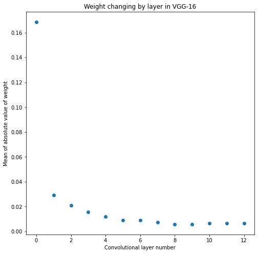
Yes, the variance does appear to drop in later layers. The biggest drop is after the first layer.
Pre-trained VGG-16 Fully Connected Layers
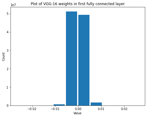
Now let’s look at the fully connected layers.
summarize(first_vgg_fc_weights, 'VGG-16', 'first fully connected', 'weights')
Shape:  (25088, 4096)
Mean:  -0.00014126883
Standard Deviation:  0.0023069018
Variance:  5.3217964e-06
Min:  -0.027062105
Max:  0.026629567

summarize(first_vgg_fc_biases, 'VGG-16', 'first fully connected', 'biases')
Shape:  (4096,)
Mean:  0.07904774
Standard Deviation:  0.18906611
Variance:  0.035745997
Min:  -0.78005254
Max:  0.8555075
summarize(last_vgg_fc_weights, 'VGG-16', 'last fully connected', 'weights')
Shape:  (4096, 1000)
Mean:  -5.3595124e-07
Standard Deviation:  0.008279975
Variance:  6.855798e-05
Min:  -0.035473574
Max:  0.057255637

summarize(last_vgg_fc_biases, 'VGG-16', 'last fully connected', 'biases')
Shape:  (1000,)
Mean:  1.4047623e-06
Standard Deviation:  0.19186237
Variance:  0.036811173
Min:  -0.773357
Max:  0.6615543
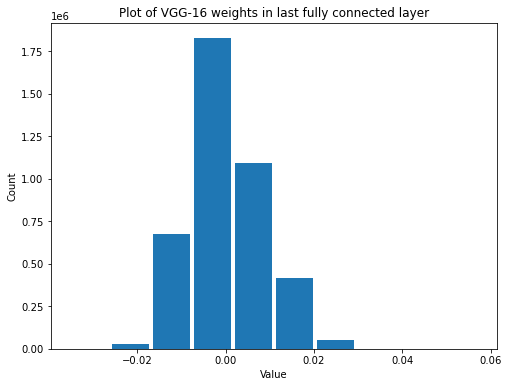
The variance increases in the layer with fewer connections, just like it did with our initialization scheme.
Now let’s look at ResNet50.
ResNet50
ResNet50 was first proposed in the paper Deep Residual Learning for Image Recognition by Kaiming He, Xiangyu Zhang, Shaoqing Ren, and Jian Sun.
resnet_model = ResNet50(weights='imagenet')
ResNet50 Convolutional Layers
Now we’ll look at a convolutional layer inside the network. I’ll just grab one from a bit deeper inside.
resnet_model.layers[25]
<tensorflow.python.keras.layers.convolutional.Conv2D at 0x16cf2609ac8>
resnet_model.layers[-6]
<tensorflow.python.keras.layers.convolutional.Conv2D at 0x16cf3b6ca88>
first_resnet_conv_weights, first_resnet_conv_biases = resnet_model.layers[2].get_weights()
mid_resnet_conv_weights, mid_resnet_conv_biases = resnet_model.layers[25].get_weights()
last_resnet_conv_weights, last_resnet_conv_biases = resnet_model.layers[-6].get_weights()
Weights and biases are not the same. Note that the first biases are basically 0.
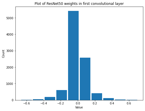
summarize(first_resnet_conv_weights, 'ResNet50', 'first convolutional', 'weights')
Shape:  (7, 7, 3, 64)
Mean:  -0.00048973627
Standard Deviation:  0.111119024
Variance:  0.012347437
Min:  -0.6710244
Max:  0.70432377

summarize(first_resnet_conv_biases, 'ResNet50', 'first convolutional', 'biases')
Shape:  (64,)
Mean:  4.5632303e-11
Standard Deviation:  2.104375e-09
Variance:  4.428394e-18
Min:  -4.4311914e-09
Max:  7.641752e-09
The biases are interesting. It appears that all the biases in the first layer are basically 0.
Now let’s look at a middle layer.
summarize(mid_resnet_conv_weights, 'ResNet50', 'middle convolutional', 'weights')
Shape:  (1, 1, 64, 256)
Mean:  -0.0009927782
Standard Deviation:  0.037277624
Variance:  0.0013896213
Min:  -0.24024516
Max:  0.27957112
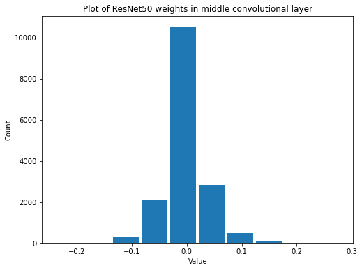
Looks like the variance has decreased by an order of magnitude. Even more of that values are close to zero now.
print_stats(mid_resnet_conv_biases)
Shape:  (256,)
Mean:  0.0
Standard Deviation:  0.0
Variance:  0.0
Min:  0.0
Max:  0.0
Wow, the biases are all completely zero here. That seems very strange to me.
summarize(last_resnet_conv_weights, 'ResNet50', 'last convolutional', 'weights')
Shape:  (1, 1, 512, 2048)
Mean:  -0.0004575059
Standard Deviation:  0.014726251
Variance:  0.00021686249
Min:  -0.1346324
Max:  0.29996708
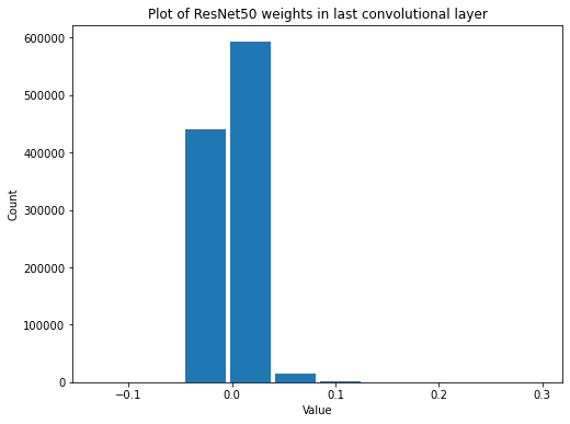
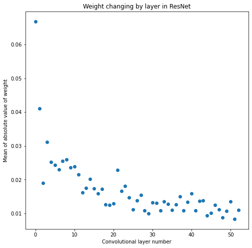
The variance has continued to shrink, again by about and order of magnitude. It looks like as you get further into the network the weights get smaller and smaller, just as we saw with VGG-16. Let’s verify that again.
resnet_conv_layers = [layer for layer in resnet_model.layers if isinstance(layer, tf.keras.layers.Conv2D)]
resnet_weight_sums = get_weight_sums(resnet_conv_layers)
plot_layer_mean_weight(resnet_weight_sums, 'ResNet')
print_stats(last_resnet_conv_biases)
Shape:  (2048,)
Mean:  0.0
Standard Deviation:  0.0
Variance:  0.0
Min:  0.0
Max:  0.0
Biases are still zero. I guess there’s just no need for them.
ResNet50 Fully Connected Layers
resnet_fc_weights, resnet_fc_biases = resnet_model.layers[-1].get_weights()
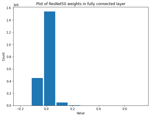
summarize(resnet_fc_weights, 'ResNet50', 'fully connected', 'weights')
Shape:  (2048, 1000)
Mean:  3.7746946e-07
Standard Deviation:  0.03353968
Variance:  0.00112491
Min:  -0.2103586
Max:  0.73615897
summarize(resnet_fc_biases, 'ResNet50', 'fully connected', 'biases')
Shape:  (1000,)
Mean:  -4.8816204e-08
Standard Deviation:  0.009334726
Variance:  8.713711e-05
Min:  -0.024051076
Max:  0.029003482

Now it looks like the biases have formed into a normal distribution.
Takeaways
There are a lot of interesting things to note from this:
- VGG weights start uniformly distributed but naturally become normally distributed
- The biases in the first convolutional layer of ResNet50 are present, but by the middle and end they are 0
- There are, however, biases in the ResNet50 fully connected layer