This tutorial shows how to plot geospatial data on a map of the US. There are lots of libraries that do all the hard work for you, so the key is just knowing that they exist and how to use them.
Table of Contents
import matplotlib.pyplot as plt
import geopandas as gpd
import pandas as pd
One of the things you’ll have to do is find the right data for mapping. Fortunately, there are datasets built into geopandas that you can use.
The key to plotting geospatial data is in shapefiles. A shapefile is a geospatial vector data format for geographic information system (GIS) software. It is used for storing the location, shape, and attributes of geographic features, such as roads, lakes, or political boundaries. A shapefile is actually a collection of files that work together. The main file (.shp) stores the geometry of the features, the index file (.shx) contains the index of the geometry, and the dBASE table (.dbf) contains attribute information for each shape. Additional files can also be included to store other types of information.
Download Map from the Internet
# Load a map of the US
us_map = gpd.read_file(gpd.datasets.get_path('naturalearth_lowres')).query('continent == "North America" and name == "United States of America"')
us_map
C:\Users\Julius\AppData\Local\Temp\ipykernel_8928\39096665.py:2: FutureWarning: The geopandas.dataset module is deprecated and will be removed in GeoPandas 1.0. You can get the original 'naturalearth_lowres' data from https://www.naturalearthdata.com/downloads/110m-cultural-vectors/.
  us_map = gpd.read_file(gpd.datasets.get_path('naturalearth_lowres')).query('continent == "North America" and name == "United States of America"')
| pop_est | continent | name | iso_a3 | gdp_md_est | geometry | |
|---|---|---|---|---|---|---|
| 4 | 328239523.0 | North America | United States of America | USA | 21433226 | MULTIPOLYGON (((-122.84000 49.00000, -120.0000... |
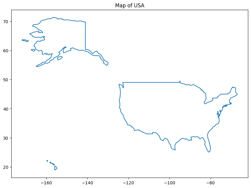
Now we can plot it.
fig, ax = plt.subplots(figsize=(10, 10))
us_map.boundary.plot(ax=ax)
ax.set_title("Map of USA")

plt.show()
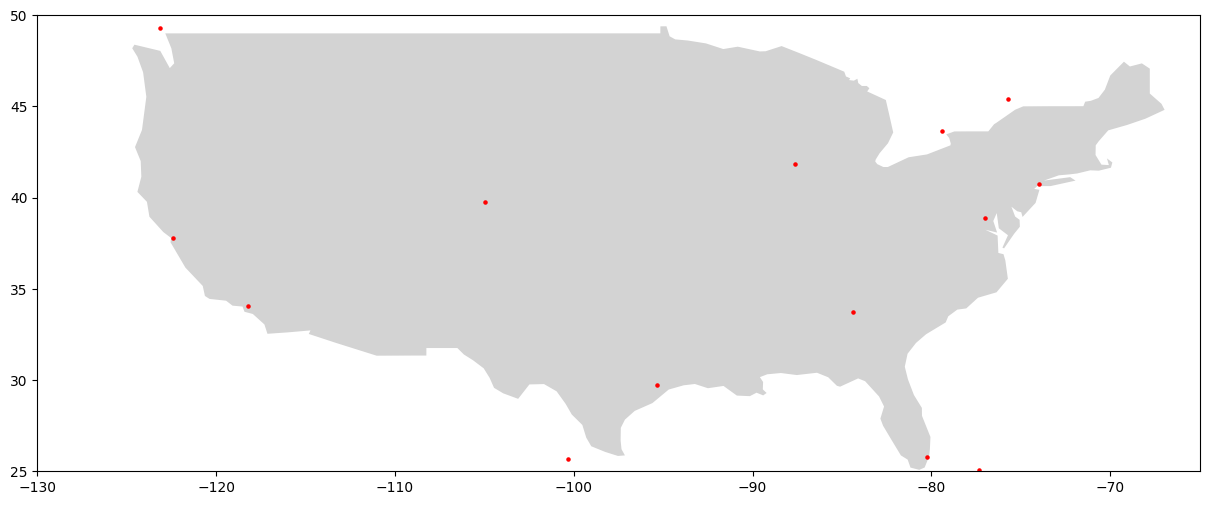
There are other datasets available, although, as you can see, they’re deprecated. But, for example, you can also get cities.
# Load the naturalearth cities dataset
cities = gpd.read_file(gpd.datasets.get_path('naturalearth_cities')) # note this is worldwide

# Plot the world map as background
fig, ax = plt.subplots(figsize=(15, 10))
us_map.plot(ax=ax, color='lightgray')

# Plot cities on top
cities.plot(ax=ax, marker='o', color='red', markersize=5)

# Focus on the US by setting the limits
ax.set_xlim([-130, -65])
ax.set_ylim([25, 50])

plt.show()
C:\Users\Julius\AppData\Local\Temp\ipykernel_8928\4049436674.py:2: FutureWarning: The geopandas.dataset module is deprecated and will be removed in GeoPandas 1.0. You can get the original 'naturalearth_cities' data from https://www.naturalearthdata.com/downloads/110m-cultural-vectors/.
  cities = gpd.read_file(gpd.datasets.get_path('naturalearth_cities')) # note this is worldwide
Use Downloaded Shapefile
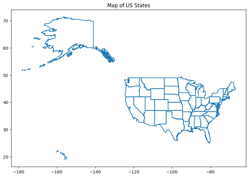
Because this is getting (unfortunately) deprecated, you might have to download your shapefiles. To use a downloaded shapefile, simply point geopandas to it.
us_states = gpd.read_file('States_shapefile-shp/States_shapefile.shp')
us_states.head()
| FID | Program | State_Code | State_Name | Flowing_St | FID_1 | geometry | |
|---|---|---|---|---|---|---|---|
| 0 | 1 | PERMIT TRACKING | AL | ALABAMA | F | 919 | POLYGON ((-85.07007 31.98070, -85.11515 31.907... |
| 1 | 2 | None | AK | ALASKA | N | 920 | MULTIPOLYGON (((-161.33379 58.73325, -161.3824... |
| 2 | 3 | AZURITE | AZ | ARIZONA | F | 921 | POLYGON ((-114.52063 33.02771, -114.55909 33.0... |
| 3 | 4 | PDS | AR | ARKANSAS | F | 922 | POLYGON ((-94.46169 34.19677, -94.45262 34.508... |
| 4 | 5 | None | CA | CALIFORNIA | N | 923 | MULTIPOLYGON (((-121.66522 38.16929, -121.7823... |
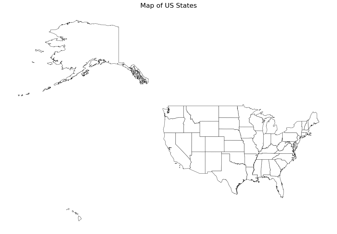
We can plot it the same way.
fig, ax = plt.subplots(figsize=(10, 10))
us_states.boundary.plot(ax=ax)
ax.set_title("Map of US States")

plt.show()
ArcGIS
You can also get data from ArcGIS.
# URL of the shapefile
url = 'https://opendata.arcgis.com/datasets/1b02c87f62d24508970dc1a6df80c98e_0.zip'

# Read the shapefile directly from the URL
states = gpd.read_file(url)

# Plot it
fig, ax = plt.subplots(figsize=(12, 8))
states.plot(ax=ax, edgecolor='black', facecolor='white', linewidth=0.5)
ax.set_title('Map of US States', fontsize=16)
ax.axis('off')
plt.tight_layout()
plt.show()
Folium
You can also use folium and Nominatim with GeoPy.
import folium
from geopy.geocoders import Nominatim
# Create a sample DataFrame with addresses
data = {
    "Address": [
        "1600 Pennsylvania Avenue NW, Washington, DC 20500",
        "One Apple Park Way, Cupertino, CA 95014",
        "1 Tesla Road, Austin, TX 78725",
        "1 Microsoft Way, Redmond, WA 98052",
        "1 Amazon Way, Seattle, WA 98109",
    ]
}
df = pd.DataFrame(data)

# Initialize the geocoder
geolocator = Nominatim(user_agent="my_app")


# Function to geocode addresses and return latitude and longitude
def geocode(address):
    location = geolocator.geocode(address)
    if location:
        return [location.latitude, location.longitude]
    return None


# Apply the geocode function to the 'Address' column
df["Coordinates"] = df["Address"].apply(geocode)

# Create a Folium map centered on the United States
map_center = [37.0902, -95.7129]  # Coordinates for the center of the US
map_zoom = 4
usa_map = folium.Map(location=map_center, zoom_start=map_zoom)

# Iterate over the DataFrame rows and add markers to the map
for _, row in df.iterrows():
    if row["Coordinates"]:
        folium.Marker(location=row["Coordinates"], popup=row["Address"]).add_to(usa_map)

# Display the map
usa_map
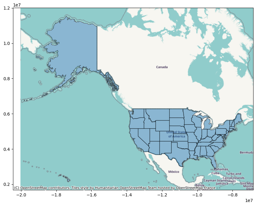
Contextily
Another option is to use contextily.
import contextily as ctx

# Ensure the CRS is compatible with web tile services
us_states_crs = us_states.to_crs(epsg=3857)

ax = us_states_crs.plot(figsize=(10, 10), alpha=0.5, edgecolor='k')
ctx.add_basemap(ax)
plt.show()