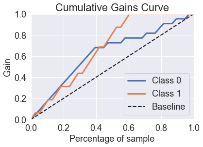
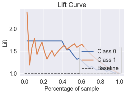
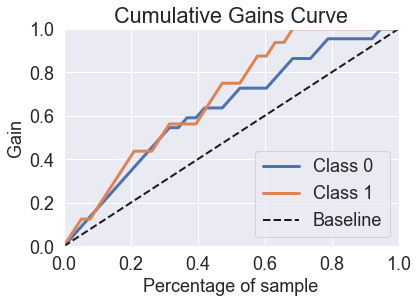
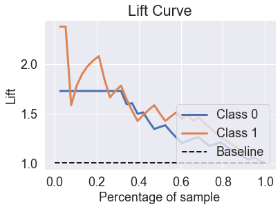
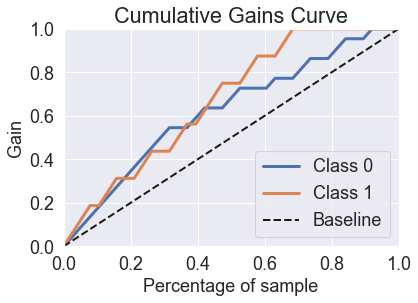
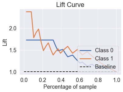
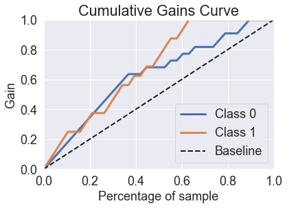
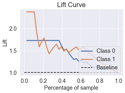
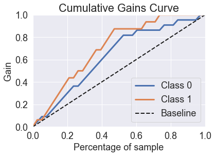
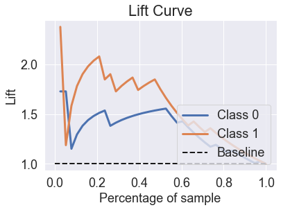
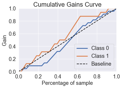
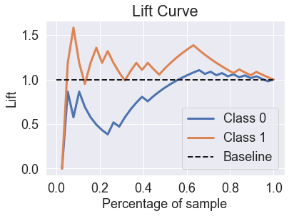
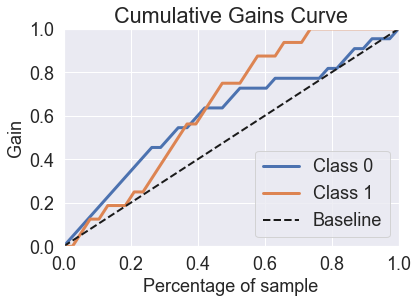
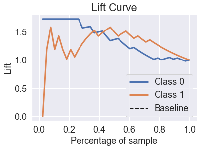
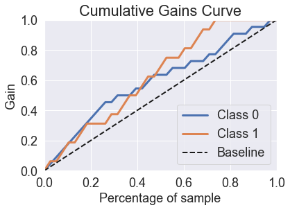
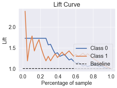
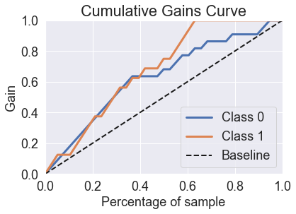
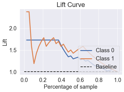
This post takes some of algorithms that we saw in the previous post and shows how they perform on the gains charts. Gains charts, which are also called lift charts, are a good way to see how much lift an algorithm has over guessing.

Table of Contents

• Data
• Algorithms
  • Gaussian Naive Bayes
  • Logistic Regression
    • Tuning the Model
  • Linear Discriminant Analysis
  • Quadratic Discriminant Analysis
  • k-Nearest Neighbors
  • Decision Trees
  • Random Forest
  • XGBoost
  • Neural Networks (Multi-layer perceptron)
    • Hyperparameter Tuning a Neural Network

import warnings

import matplotlib.pyplot as plt
import numpy as np
import pandas as pd
import scikitplot as skplt
import seaborn as sns
import xgboost as xgb
from mlxtend.plotting import plot_decision_regions
from sklearn import metrics, model_selection
from sklearn.discriminant_analysis import LinearDiscriminantAnalysis, QuadraticDiscriminantAnalysis
from sklearn.ensemble import RandomForestClassifier
from sklearn.linear_model import LogisticRegression
from sklearn.model_selection import GridSearchCV, train_test_split
from sklearn.naive_bayes import GaussianNB
from sklearn.neighbors import KNeighborsClassifier
from sklearn.neural_network import MLPClassifier
from sklearn.preprocessing import StandardScaler
from sklearn.tree import DecisionTreeClassifier

warnings.filterwarnings("ignore")
sns.set(font_scale=1.5)

Data

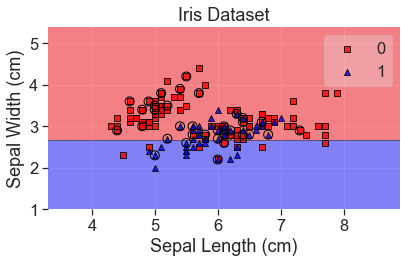
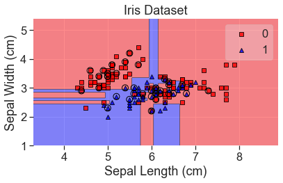
df = sns.load_dataset("iris")

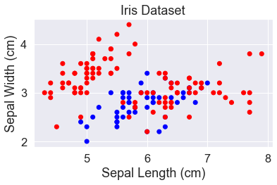
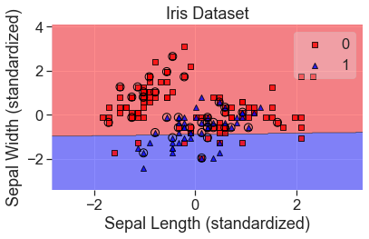
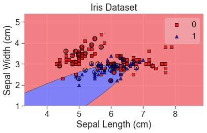
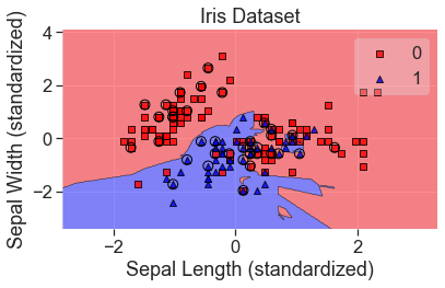
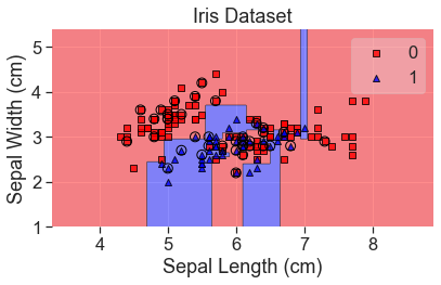
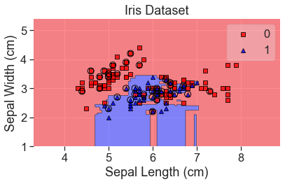
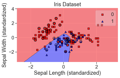
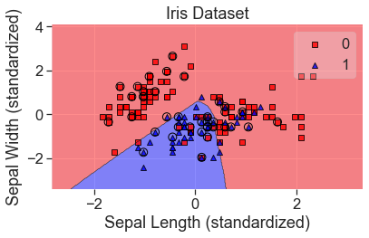
We’ll keep using the iris dataset. Last time we looked at petal length and petal width because they provided good separation between this classes. This time we’ll look at sepal length and sepal width to make it more challenging for the classifiers.

Most everything else is the same as last time, so I won’t go into much detail here.

X = df[['sepal_length', 'sepal_width']]
y = df['species']
# change the labels to numbers
y = pd.factorize(y, sort=True)[0]

In this case, we’re going to build an algorithm to determine whether an iris is the versicolor species. This will allow us to use lift and gain charts to analyze our results.

y = (y == 1).astype(int)

X_train, X_test, y_train, y_test = train_test_split(
    X, y, test_size=0.25, random_state=0, shuffle=True
)

# Convert the pandas dataframes to numpy arrays
X_array = np.asarray(X)
X_train_array = np.asarray(X_train)
X_test_array = np.asarray(X_test)

def add_labels(standardized=False):
    plt.title('Iris Dataset')
    if standardized:
        plt.xlabel('Sepal Length (standardized)')
        plt.ylabel('Sepal Width (standardized)')
    else:
        plt.xlabel('Sepal Length (cm)')
        plt.ylabel('Sepal Width (cm)')
    plt.tight_layout()
    plt.show()

y_str = y.astype(str)
y_str[y_str == '0'] = 'red'
y_str[y_str == '1'] = 'blue'

plt.scatter(X['sepal_length'], X['sepal_width'], c=y_str)
add_labels()

Algorithms

Gaussian Naive Bayes

gnb = GaussianNB()
gnb.fit(X_train, y_train)
print(
    "{:.1%} of the test set was correct.".format(
        metrics.accuracy_score(y_test, gnb.predict(X_test))
    )
)

71.1% of the test set was correct.

predicted_probas_gnb = gnb.predict_proba(X_test)

def show_scores(preds, y_true):
    sorted_preds, sorted_y_true = zip(*sorted(zip(preds, y_true), reverse=True))
    for i, label in enumerate(sorted_y_true):
        print(f"Label: {label}, Prediction: {round(sorted_preds[i], 4)}")

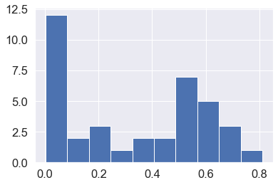
We can sometimes get a better since of what’s going on by looking at the raw scores.

show_scores(predicted_probas_gnb[:,1], y_test)

Label: 1, Prediction: 0.8117
Label: 0, Prediction: 0.7047
Label: 1, Prediction: 0.6649
Label: 1, Prediction: 0.6568
Label: 0, Prediction: 0.6034
Label: 1, Prediction: 0.6003
Label: 1, Prediction: 0.6003
Label: 0, Prediction: 0.5861
Label: 0, Prediction: 0.5723
Label: 1, Prediction: 0.5444
Label: 1, Prediction: 0.5402
Label: 0, Prediction: 0.5369
Label: 1, Prediction: 0.5323
Label: 1, Prediction: 0.5176
Label: 1, Prediction: 0.5017
Label: 1, Prediction: 0.4882
Label: 0, Prediction: 0.4555
Label: 1, Prediction: 0.4269
Label: 1, Prediction: 0.37
Label: 1, Prediction: 0.3588
Label: 0, Prediction: 0.3151
Label: 1, Prediction: 0.2413
Label: 1, Prediction: 0.2173
Label: 0, Prediction: 0.1929
Label: 0, Prediction: 0.1298
Label: 0, Prediction: 0.0844
Label: 0, Prediction: 0.0535
Label: 0, Prediction: 0.0535
Label: 0, Prediction: 0.0533
Label: 0, Prediction: 0.045
Label: 0, Prediction: 0.0344
Label: 0, Prediction: 0.0311
Label: 0, Prediction: 0.0223
Label: 0, Prediction: 0.0164
Label: 0, Prediction: 0.0094
Label: 0, Prediction: 0.0092
Label: 0, Prediction: 0.0063
Label: 0, Prediction: 0.0015

plt.hist(predicted_probas_gnb[:,1]);

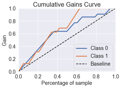
skplt.metrics.plot_cumulative_gain(y_test, predicted_probas_gnb);

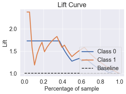
skplt.metrics.plot_lift_curve(y_test, predicted_probas_gnb);

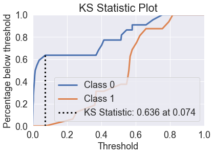
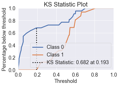
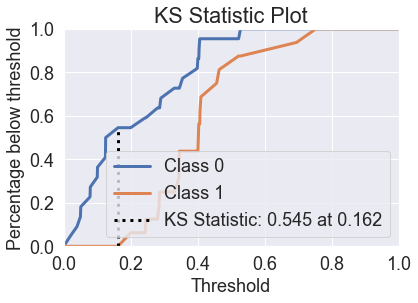
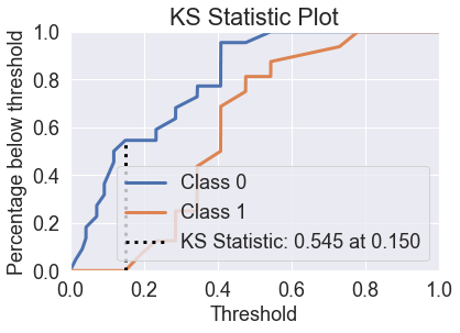
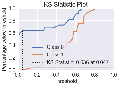
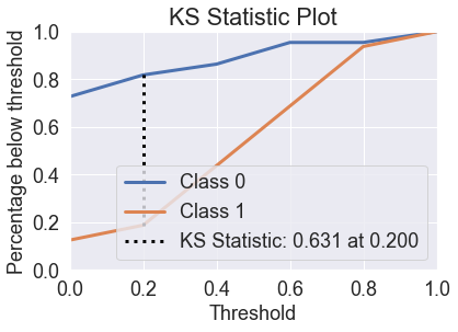
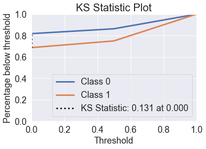
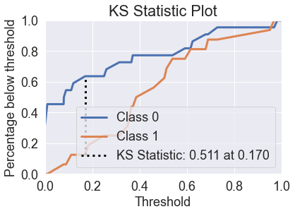
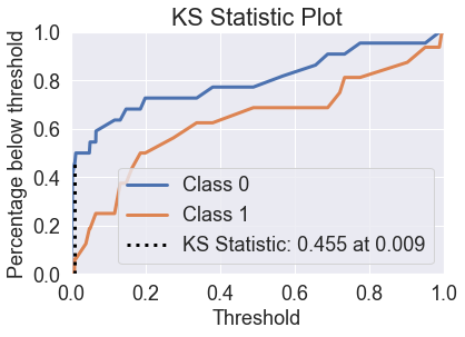
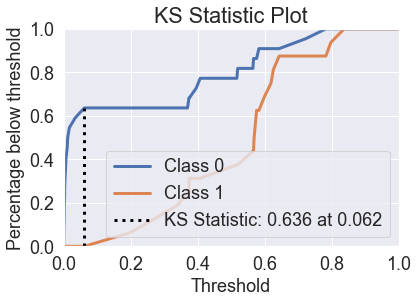
skplt.metrics.plot_ks_statistic(y_test, predicted_probas_gnb);

Logistic Regression

scale = StandardScaler()
scale.fit(X_train)
X_std = scale.transform(X)
X_train_std = scale.transform(X_train)
X_test_std = scale.transform(X_test)

lgr = LogisticRegression(solver="lbfgs", multi_class="auto")
lgr.fit(X_train_std, y_train)
print(
    "{:.1%} of the test set was correct.".format(
        metrics.accuracy_score(y_test, lgr.predict(X_test_std))
    )
)

63.2% of the test set was correct.

plot_decision_regions(
    X_std, y, clf=lgr, X_highlight=X_test_std, colors='red,blue'
)
add_labels(standardized=True)

predicted_probas_lgr = lgr.predict_proba(X_test_std)
skplt.metrics.plot_cumulative_gain(y_test, predicted_probas_lgr);

skplt.metrics.plot_lift_curve(y_test, predicted_probas_lgr);

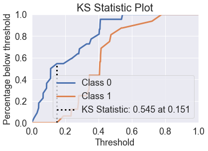
skplt.metrics.plot_ks_statistic(y_test, predicted_probas_lgr);

Tuning the Model

C_grid = np.logspace(-3, 3, 10)
max_iter_grid = np.logspace(2,3,6)
hyperparameters = dict(C=C_grid, max_iter=max_iter_grid)
lgr_grid = GridSearchCV(lgr, hyperparameters, cv=3)

# Re-fit and test after optimizing
lgr_grid.fit(X_train_std, y_train)
print(
    "{:.1%} of the test set was correct.".format(
        metrics.accuracy_score(y_test, lgr_grid.predict(X_test_std))
    )
)

63.2% of the test set was correct.

print(lgr_grid.best_estimator_)

LogisticRegression(C=0.46415888336127775, max_iter=100.0)

plot_decision_regions(
    X_std, y, clf=lgr_grid, X_highlight=X_test_std, colors='red,blue'
)
add_labels(standardized=True)

predicted_probas_lgr_grid = lgr_grid.predict_proba(X_test_std)
skplt.metrics.plot_cumulative_gain(y_test, predicted_probas_lgr_grid);

skplt.metrics.plot_lift_curve(y_test, predicted_probas_lgr_grid);

skplt.metrics.plot_ks_statistic(y_test, predicted_probas_lgr_grid);

Linear Discriminant Analysis

lda = LinearDiscriminantAnalysis()
lda.fit(X_train, y_train)
print(
    "{:.1%} of the test set was correct.".format(
        metrics.accuracy_score(y_test, lda.predict(X_test))
    )
)

63.2% of the test set was correct.

plot_decision_regions(
    X_array, y, clf=lda, X_highlight=X_test_array, colors='red,blue'
)
add_labels()

predicted_probas_lda = lda.predict_proba(X_test)
skplt.metrics.plot_cumulative_gain(y_test, predicted_probas_lda)
plt.show()

skplt.metrics.plot_lift_curve(y_test, predicted_probas_lda);

skplt.metrics.plot_ks_statistic(y_test, predicted_probas_lda);

Quadratic Discriminant Analysis

qda = QuadraticDiscriminantAnalysis()
qda.fit(X_train, y_train)
metrics.accuracy_score(y_test, qda.predict(X_test))

0.6842105263157895

plot_decision_regions(
    X_array, y, clf=qda, X_highlight=X_test_array, colors='red,blue'
)
add_labels()

predicted_probas_qda = qda.predict_proba(X_test)
skplt.metrics.plot_cumulative_gain(y_test, predicted_probas_qda)
plt.show()

skplt.metrics.plot_lift_curve(y_test, predicted_probas_qda);

skplt.metrics.plot_ks_statistic(y_test, predicted_probas_qda);

show_scores(predicted_probas_qda[:,1], y_test)

Label: 1, Prediction: 0.8297
Label: 1, Prediction: 0.7378
Label: 1, Prediction: 0.6914
Label: 1, Prediction: 0.6888
Label: 0, Prediction: 0.686
Label: 0, Prediction: 0.6362
Label: 1, Prediction: 0.6322
Label: 1, Prediction: 0.6322
Label: 0, Prediction: 0.6107
Label: 0, Prediction: 0.5881
Label: 1, Prediction: 0.5796
Label: 1, Prediction: 0.5792
Label: 1, Prediction: 0.5695
Label: 0, Prediction: 0.5345
Label: 1, Prediction: 0.5104
Label: 0, Prediction: 0.5083
Label: 1, Prediction: 0.4794
Label: 0, Prediction: 0.4325
Label: 1, Prediction: 0.3676
Label: 1, Prediction: 0.3525
Label: 1, Prediction: 0.3416
Label: 0, Prediction: 0.2779
Label: 1, Prediction: 0.2687
Label: 1, Prediction: 0.2257
Label: 0, Prediction: 0.0471
Label: 0, Prediction: 0.0181
Label: 0, Prediction: 0.0039
Label: 0, Prediction: 0.0012
Label: 0, Prediction: 0.0012
Label: 0, Prediction: 0.001
Label: 0, Prediction: 0.001
Label: 0, Prediction: 0.0003
Label: 0, Prediction: 0.0002
Label: 0, Prediction: 0.0
Label: 0, Prediction: 0.0
Label: 0, Prediction: 0.0
Label: 0, Prediction: 0.0
Label: 0, Prediction: 0.0

k-Nearest Neighbors

knn = KNeighborsClassifier()
knn.fit(X_train_std, y_train)
print(
    "{:.1%} of the test set was correct.".format(
        metrics.accuracy_score(y_test, knn.predict(X_test_std))
    )
)

73.7% of the test set was correct.

plot_decision_regions(
    X_std, y, clf=knn, X_highlight=X_test_std, colors='red,blue'
)
add_labels(standardized=True)

predicted_probas_knn = knn.predict_proba(X_test_std)
skplt.metrics.plot_cumulative_gain(y_test, predicted_probas_knn);

skplt.metrics.plot_lift_curve(y_test, predicted_probas_knn);

skplt.metrics.plot_ks_statistic(y_test, predicted_probas_knn);

Decision Trees

tre = DecisionTreeClassifier(random_state=0)
tre.fit(X_train, y_train)
print(
    "{:.1%} of the test set was correct.".format(
        metrics.accuracy_score(y_test, tre.predict(X_test))
    ))

60.5% of the test set was correct.

plot_decision_regions(
    X_array, y, clf=tre, X_highlight=X_test_array, colors='red,blue'
)
add_labels()

predicted_probas_tre = tre.predict_proba(X_test)
skplt.metrics.plot_cumulative_gain(y_test, predicted_probas_tre)
plt.show()

skplt.metrics.plot_lift_curve(y_test, predicted_probas_tre);

skplt.metrics.plot_ks_statistic(y_test, predicted_probas_tre);

You’ll see that decision trees perform quite poorly in these charts. If we look at the probabilities, you can see why.

show_scores(predicted_probas_tre[:,1], y_test)

Label: 1, Prediction: 1.0
Label: 1, Prediction: 1.0
Label: 1, Prediction: 1.0
Label: 1, Prediction: 1.0
Label: 0, Prediction: 1.0
Label: 0, Prediction: 1.0
Label: 0, Prediction: 1.0
Label: 1, Prediction: 0.5
Label: 0, Prediction: 0.5
Label: 1, Prediction: 0.0
Label: 1, Prediction: 0.0
Label: 1, Prediction: 0.0
Label: 1, Prediction: 0.0
Label: 1, Prediction: 0.0
Label: 1, Prediction: 0.0
Label: 1, Prediction: 0.0
Label: 1, Prediction: 0.0
Label: 1, Prediction: 0.0
Label: 1, Prediction: 0.0
Label: 1, Prediction: 0.0
Label: 0, Prediction: 0.0
Label: 0, Prediction: 0.0
Label: 0, Prediction: 0.0
Label: 0, Prediction: 0.0
Label: 0, Prediction: 0.0
Label: 0, Prediction: 0.0
Label: 0, Prediction: 0.0
Label: 0, Prediction: 0.0
Label: 0, Prediction: 0.0
Label: 0, Prediction: 0.0
Label: 0, Prediction: 0.0
Label: 0, Prediction: 0.0
Label: 0, Prediction: 0.0
Label: 0, Prediction: 0.0
Label: 0, Prediction: 0.0
Label: 0, Prediction: 0.0
Label: 0, Prediction: 0.0
Label: 0, Prediction: 0.0

Random Forest

rfc = RandomForestClassifier(random_state=0)
rfc.fit(X_train, y_train)
print(
    "{:.1%} of the test set was correct.".format(
        metrics.accuracy_score(y_test, rfc.predict(X_test))
    ))

63.2% of the test set was correct.

plot_decision_regions(
    X_array, y, clf=rfc, X_highlight=X_test_array, colors='red,blue'
)
add_labels()

predicted_probas_rfc = rfc.predict_proba(X_test)
skplt.metrics.plot_cumulative_gain(y_test, predicted_probas_rfc)
plt.show()

skplt.metrics.plot_lift_curve(y_test, predicted_probas_rfc);

skplt.metrics.plot_ks_statistic(y_test, predicted_probas_rfc);

The random forest is able to fix the prediction problems that were caused by using a single decision tree.

show_scores(predicted_probas_rfc[:,1], y_test)

Label: 0, Prediction: 0.9833
Label: 1, Prediction: 0.97
Label: 1, Prediction: 0.9517
Label: 0, Prediction: 0.7295
Label: 1, Prediction: 0.69
Label: 0, Prediction: 0.68
Label: 0, Prediction: 0.6248
Label: 1, Prediction: 0.6163
Label: 0, Prediction: 0.5927
Label: 1, Prediction: 0.5395
Label: 1, Prediction: 0.5148
Label: 1, Prediction: 0.5052
Label: 1, Prediction: 0.46
Label: 1, Prediction: 0.3861
Label: 0, Prediction: 0.3715
Label: 1, Prediction: 0.3658
Label: 1, Prediction: 0.3658
Label: 1, Prediction: 0.35
Label: 0, Prediction: 0.315
Label: 0, Prediction: 0.26
Label: 1, Prediction: 0.25
Label: 1, Prediction: 0.1833
Label: 0, Prediction: 0.17
Label: 0, Prediction: 0.12
Label: 1, Prediction: 0.111
Label: 0, Prediction: 0.0892
Label: 0, Prediction: 0.08
Label: 1, Prediction: 0.0792
Label: 0, Prediction: 0.01
Label: 0, Prediction: 0.01
Label: 0, Prediction: 0.01
Label: 0, Prediction: 0.0
Label: 0, Prediction: 0.0
Label: 0, Prediction: 0.0
Label: 0, Prediction: 0.0
Label: 0, Prediction: 0.0
Label: 0, Prediction: 0.0
Label: 0, Prediction: 0.0

XGBoost

xg = xgb.XGBClassifier(random_state=42)

xg.fit(X_train, y_train)
print(
    "{:.1%} of the test set was correct.".format(
        metrics.accuracy_score(y_test, xg.predict(X_test))
    ))

57.9% of the test set was correct.

plot_decision_regions(
    X_array, y, clf=xg, X_highlight=X_test_array, colors='red,blue'
)
add_labels()

predicted_probas_xg = xg.predict_proba(X_test)
skplt.metrics.plot_cumulative_gain(y_test, predicted_probas_xg)
plt.show()

skplt.metrics.plot_lift_curve(y_test, predicted_probas_xg);

skplt.metrics.plot_ks_statistic(y_test, predicted_probas_xg);

show_scores(predicted_probas_xg[:,1], y_test)

Label: 1, Prediction: 0.9961000084877014
Label: 0, Prediction: 0.989300012588501
Label: 1, Prediction: 0.9514999985694885
Label: 1, Prediction: 0.9035000205039978
Label: 0, Prediction: 0.7764000296592712
Label: 1, Prediction: 0.7348999977111816
Label: 1, Prediction: 0.722100019454956
Label: 0, Prediction: 0.6895999908447266
Label: 0, Prediction: 0.6570000052452087
Label: 0, Prediction: 0.5684999823570251
Label: 1, Prediction: 0.49000000953674316
Label: 0, Prediction: 0.38089999556541443
Label: 1, Prediction: 0.337799996137619
Label: 1, Prediction: 0.2752000093460083
Label: 0, Prediction: 0.1995999962091446
Label: 1, Prediction: 0.1867000013589859
Label: 1, Prediction: 0.16410000622272491
Label: 0, Prediction: 0.14830000698566437
Label: 1, Prediction: 0.13259999454021454
Label: 1, Prediction: 0.13259999454021454
Label: 0, Prediction: 0.11749999970197678
Label: 0, Prediction: 0.06750000268220901
Label: 1, Prediction: 0.06689999997615814
Label: 0, Prediction: 0.051600001752376556
Label: 1, Prediction: 0.04969999939203262
Label: 1, Prediction: 0.040300000458955765
Label: 0, Prediction: 0.013299999758601189
Label: 1, Prediction: 0.010400000028312206
Label: 0, Prediction: 0.00930000003427267
Label: 0, Prediction: 0.004000000189989805
Label: 0, Prediction: 0.004000000189989805
Label: 0, Prediction: 0.004000000189989805
Label: 0, Prediction: 0.003800000064074993
Label: 0, Prediction: 0.003800000064074993
Label: 0, Prediction: 0.002099999925121665
Label: 0, Prediction: 0.0019000000320374966
Label: 0, Prediction: 0.0019000000320374966
Label: 0, Prediction: 0.0019000000320374966

Neural Networks (Multi-layer perceptron)

mlp = MLPClassifier(max_iter=500)
mlp.fit(X_train_std, y_train)
print(
    "{:.1%} of the test set was correct.".format(
        metrics.accuracy_score(y_test, mlp.predict(X_test_std))
    )
)

73.7% of the test set was correct.

plot_decision_regions(
    X_std, y, clf=mlp, X_highlight=X_test_std, colors='red,blue'
)
add_labels(standardized=True)

predicted_probas_mlp = mlp.predict_proba(X_test_std)
skplt.metrics.plot_cumulative_gain(y_test, predicted_probas_mlp)
plt.show()

skplt.metrics.plot_lift_curve(y_test, predicted_probas_mlp);

skplt.metrics.plot_ks_statistic(y_test, predicted_probas_mlp);

show_scores(predicted_probas_mlp[:,1], y_test)

Label: 1, Prediction: 0.8378
Label: 1, Prediction: 0.7979
Label: 0, Prediction: 0.7831
Label: 0, Prediction: 0.7228
Label: 1, Prediction: 0.6435
Label: 1, Prediction: 0.6263
Label: 1, Prediction: 0.6191
Label: 1, Prediction: 0.5993
Label: 0, Prediction: 0.5829
Label: 1, Prediction: 0.5762
Label: 1, Prediction: 0.5762
Label: 1, Prediction: 0.5687
Label: 0, Prediction: 0.5669
Label: 1, Prediction: 0.5652
Label: 0, Prediction: 0.5197
Label: 1, Prediction: 0.5173
Label: 0, Prediction: 0.4077
Label: 0, Prediction: 0.3957
Label: 1, Prediction: 0.375
Label: 0, Prediction: 0.374
Label: 1, Prediction: 0.3698
Label: 1, Prediction: 0.3395
Label: 1, Prediction: 0.2695
Label: 1, Prediction: 0.1982
Label: 0, Prediction: 0.0616
Label: 0, Prediction: 0.0345
Label: 0, Prediction: 0.0169
Label: 0, Prediction: 0.0119
Label: 0, Prediction: 0.0105
Label: 0, Prediction: 0.0072
Label: 0, Prediction: 0.0072
Label: 0, Prediction: 0.0041
Label: 0, Prediction: 0.0029
Label: 0, Prediction: 0.0028
Label: 0, Prediction: 0.0016
Label: 0, Prediction: 0.0014
Label: 0, Prediction: 0.0008
Label: 0, Prediction: 0.0005

Hyperparameter Tuning a Neural Network

alpha_grid = np.logspace(-5, 3, 5)
learning_rate_init_grid = np.logspace(-6, -2, 5)
max_iter_grid = [200, 2000]
hyperparameters = dict(
    alpha=alpha_grid, learning_rate_init=learning_rate_init_grid, max_iter=max_iter_grid
)
mlp_grid = GridSearchCV(mlp, hyperparameters)

mlp_grid.fit(X_train_std, y_train)
print(
    "{:.1%} of the test set was correct.".format(
        metrics.accuracy_score(y_test, mlp.predict(X_test_std))
    )
)

73.7% of the test set was correct.

print(mlp_grid.best_estimator_)

MLPClassifier(alpha=0.1, max_iter=2000)

plot_decision_regions(
    X_std, y, clf=mlp_grid, X_highlight=X_test_std, colors='red,blue'
)
add_labels(standardized=True)

predicted_probas_mlp_grid = mlp_grid.predict_proba(X_test_std)
skplt.metrics.plot_cumulative_gain(y_test, predicted_probas_mlp_grid)
plt.show()

skplt.metrics.plot_lift_curve(y_test, predicted_probas_mlp_grid);

skplt.metrics.plot_ks_statistic(y_test, predicted_probas_mlp_grid);