
In this notebook, I’m going to look at the basics of cleaning data with Python. I will be using a dataset of people involved in the Enron scandal. I first saw this dataset in the Intro to Machine Learning class at Udacity.
Table of Contents
# Imports
import pickle
from os.path import join

import matplotlib
import matplotlib.pyplot as plt
import numpy as np
import pandas as pd
Loading the Data
The first step is to load the data. It’s saved as a pickle file, which is a filetype created by the pickle module - a Python module to efficiently serialize and de-serialize data. Serializing is a process of converting a Python data object, like a list or dictionary, into a stream of characters.
path = "datasets/Enron/"
file = "final_project_dataset.pkl"
with open(join(path, file), "rb") as f:
    enron_data = pickle.load(f)
Note that this repository does not include the Enron data files. Download final_project_dataset.pkl (for example from Udacity’s machine learning mini-projects) and place it in datasets/Enron/ so the code above can load it.
Exploring the Data
Now let’s look at the data. First, we’ll see what type it is.
print("The dataset is a", type(enron_data))
The dataset is a <class 'dict'>
OK, we have a dictionary. That means we’ll have to find the values by calling the associated keys. Let’s see what different keys we have in the dataset.
print("There are {} entities in the dataset.\n".format(len(enron_data)))
print(enron_data.keys())
There are 146 entities in the dataset.

dict_keys(['METTS MARK', 'BAXTER JOHN C', 'ELLIOTT STEVEN', 'CORDES WILLIAM R', 'HANNON KEVIN P', 'MORDAUNT KRISTINA M', 'MEYER ROCKFORD G', 'MCMAHON JEFFREY', 'HAEDICKE MARK E', 'PIPER GREGORY F', 'HUMPHREY GENE E', 'NOLES JAMES L', 'BLACHMAN JEREMY M', 'SUNDE MARTIN', 'GIBBS DANA R', 'LOWRY CHARLES P', 'COLWELL WESLEY', 'MULLER MARK S', 'JACKSON CHARLENE R', 'WESTFAHL RICHARD K', 'WALTERS GARETH W', 'WALLS JR ROBERT H', 'KITCHEN LOUISE', 'CHAN RONNIE', 'BELFER ROBERT', 'SHANKMAN JEFFREY A', 'WODRASKA JOHN', 'BERGSIEKER RICHARD P', 'URQUHART JOHN A', 'BIBI PHILIPPE A', 'RIEKER PAULA H', 'WHALEY DAVID A', 'BECK SALLY W', 'HAUG DAVID L', 'ECHOLS JOHN B', 'MENDELSOHN JOHN', 'HICKERSON GARY J', 'CLINE KENNETH W', 'LEWIS RICHARD', 'HAYES ROBERT E', 'KOPPER MICHAEL J', 'LEFF DANIEL P', 'LAVORATO JOHN J', 'BERBERIAN DAVID', 'DETMERING TIMOTHY J', 'WAKEHAM JOHN', 'POWERS WILLIAM', 'GOLD JOSEPH', 'BANNANTINE JAMES M', 'DUNCAN JOHN H', 'SHAPIRO RICHARD S', 'SHERRIFF JOHN R', 'SHELBY REX', 'LEMAISTRE CHARLES', 'DEFFNER JOSEPH M', 'KISHKILL JOSEPH G', 'WHALLEY LAWRENCE G', 'MCCONNELL MICHAEL S', 'PIRO JIM', 'DELAINEY DAVID W', 'SULLIVAN-SHAKLOVITZ COLLEEN', 'WROBEL BRUCE', 'LINDHOLM TOD A', 'MEYER JEROME J', 'LAY KENNETH L', 'BUTTS ROBERT H', 'OLSON CINDY K', 'MCDONALD REBECCA', 'CUMBERLAND MICHAEL S', 'GAHN ROBERT S', 'BADUM JAMES P', 'HERMANN ROBERT J', 'FALLON JAMES B', 'GATHMANN WILLIAM D', 'HORTON STANLEY C', 'BOWEN JR RAYMOND M', 'GILLIS JOHN', 'FITZGERALD JAY L', 'MORAN MICHAEL P', 'REDMOND BRIAN L', 'BAZELIDES PHILIP J', 'BELDEN TIMOTHY N', 'DIMICHELE RICHARD G', 'DURAN WILLIAM D', 'THORN TERENCE H', 'FASTOW ANDREW S', 'FOY JOE', 'CALGER CHRISTOPHER F', 'RICE KENNETH D', 'KAMINSKI WINCENTY J', 'LOCKHART EUGENE E', 'COX DAVID', 'OVERDYKE JR JERE C', 'PEREIRA PAULO V. FERRAZ', 'STABLER FRANK', 'SKILLING JEFFREY K', 'BLAKE JR. NORMAN P', 'SHERRICK JEFFREY B', 'PRENTICE JAMES', 'GRAY RODNEY', 'THE TRAVEL AGENCY IN THE PARK', 'UMANOFF ADAM S', 'KEAN STEVEN J', 'TOTAL', 'FOWLER PEGGY', 'WASAFF GEORGE', 'WHITE JR THOMAS E', 'CHRISTODOULOU DIOMEDES', 'ALLEN PHILLIP K', 'SHARP VICTORIA T', 'JAEDICKE ROBERT', 'WINOKUR JR. HERBERT S', 'BROWN MICHAEL', 'MCCLELLAN GEORGE', 'HUGHES JAMES A', 'REYNOLDS LAWRENCE', 'PICKERING MARK R', 'BHATNAGAR SANJAY', 'CARTER REBECCA C', 'BUCHANAN HAROLD G', 'YEAP SOON', 'MURRAY JULIA H', 'GARLAND C KEVIN', 'DODSON KEITH', 'YEAGER F SCOTT', 'HIRKO JOSEPH', 'DIETRICH JANET R', 'DERRICK JR. JAMES V', 'FREVERT MARK A', 'PAI LOU L', 'HAYSLETT RODERICK J', 'BAY FRANKLIN R', 'MCCARTY DANNY J', 'FUGH JOHN L', 'SCRIMSHAW MATTHEW', 'KOENIG MARK E', 'SAVAGE FRANK', 'IZZO LAWRENCE L', 'TILNEY ELIZABETH A', 'MARTIN AMANDA K', 'BUY RICHARD B', 'GRAMM WENDY L', 'CAUSEY RICHARD A', 'TAYLOR MITCHELL S', 'DONAHUE JR JEFFREY M', 'GLISAN JR BEN F'])
The keys are different people who worked at Enron. I see several names familiar from the Enron scandal, including Kenneth Lay, Jeffery Skilling, Andrew Fastow, and Cliff Baxter (who’s listed as John C Baxter). There’s also an entity named “The Travel Agency in the Park”. From footnote j in the original document, this business was co-owned by the sister of Enron’s former Chairman. It may be of interest to investigators, but it will mess up the machine learning algorithms as it’s not an employee, so I will remove it.
Now let’s see what information we have about each person. We’ll start with Ken Lay.
enron_data["LAY KENNETH L"]
{'salary': 1072321,
 'to_messages': 4273,
 'deferral_payments': 202911,
 'total_payments': 103559793,
 'loan_advances': 81525000,
 'bonus': 7000000,
 'email_address': 'kenneth.lay@enron.com',
 'restricted_stock_deferred': 'NaN',
 'deferred_income': -300000,
 'total_stock_value': 49110078,
 'expenses': 99832,
 'from_poi_to_this_person': 123,
 'exercised_stock_options': 34348384,
 'from_messages': 36,
 'other': 10359729,
 'from_this_person_to_poi': 16,
 'poi': True,
 'long_term_incentive': 3600000,
 'shared_receipt_with_poi': 2411,
 'restricted_stock': 14761694,
 'director_fees': 'NaN'}
There are checksums built into the dataset, like total_payments and total_stock_value. We should be able to calculate these from the other values to double-check the values.
We can also query for a specific value, like this:
print("Jeff Skilling's total payments were ${:,.0f}.".format(enron_data["SKILLING JEFFREY K"]["total_payments"]))
Jeff Skilling's total payments were $8,682,716.
Before we go any further, we’ll put the data into a pandas DataFrame to make it easier to work with.
# The keys of the dictionary are the people, so we'll want them to be the rows of the dataframe
df = pd.DataFrame.from_dict(enron_data, orient="index")
pd.set_option("display.max_columns", len(df.columns))
df.head()
| salary | to_messages | deferral_payments | total_payments | loan_advances | bonus | email_address | restricted_stock_deferred | deferred_income | total_stock_value | expenses | from_poi_to_this_person | exercised_stock_options | from_messages | other | from_this_person_to_poi | poi | long_term_incentive | shared_receipt_with_poi | restricted_stock | director_fees | |
|---|---|---|---|---|---|---|---|---|---|---|---|---|---|---|---|---|---|---|---|---|---|
| METTS MARK | 365788 | 807 | NaN | 1061827 | NaN | 600000 | mark.metts@enron.com | NaN | NaN | 585062 | 94299 | 38 | NaN | 29 | 1740 | 1 | False | NaN | 702 | 585062 | NaN |
| BAXTER JOHN C | 267102 | NaN | 1295738 | 5634343 | NaN | 1200000 | NaN | NaN | -1386055 | 10623258 | 11200 | NaN | 6680544 | NaN | 2660303 | NaN | False | 1586055 | NaN | 3942714 | NaN |
| ELLIOTT STEVEN | 170941 | NaN | NaN | 211725 | NaN | 350000 | steven.elliott@enron.com | NaN | -400729 | 6678735 | 78552 | NaN | 4890344 | NaN | 12961 | NaN | False | NaN | NaN | 1788391 | NaN |
| CORDES WILLIAM R | NaN | 764 | NaN | NaN | NaN | NaN | bill.cordes@enron.com | NaN | NaN | 1038185 | NaN | 10 | 651850 | 12 | NaN | 0 | False | NaN | 58 | 386335 | NaN |
| HANNON KEVIN P | 243293 | 1045 | NaN | 288682 | NaN | 1500000 | kevin.hannon@enron.com | NaN | -3117011 | 6391065 | 34039 | 32 | 5538001 | 32 | 11350 | 21 | True | 1617011 | 1035 | 853064 | NaN |
Sometimes it can be helpful to export the data to a spreadsheet. If you want to do that, you can do it like so:
df.to_csv('final_project_dataset.csv')
We can already see missing values, and it looks like they’re entered as NaN, which Python will see as a string and not recognize as a null value. We can do a quick replacement on those.
df = df.replace("NaN", np.nan)
Pandas makes summarizing the data simple. First, we’ll configure pandas to print in standard notation with no decimal places.
pd.options.display.float_format = "{:10,.0f}".format
df.describe()
| salary | to_messages | deferral_payments | total_payments | loan_advances | bonus | restricted_stock_deferred | deferred_income | total_stock_value | expenses | from_poi_to_this_person | exercised_stock_options | from_messages | other | from_this_person_to_poi | long_term_incentive | shared_receipt_with_poi | restricted_stock | director_fees | |
|---|---|---|---|---|---|---|---|---|---|---|---|---|---|---|---|---|---|---|---|
| count | 95 | 86 | 39 | 125 | 4 | 82 | 18 | 49 | 126 | 95 | 86 | 102 | 86 | 93 | 86 | 66 | 86 | 110 | 17 |
| mean | 562,194 | 2,074 | 1,642,674 | 5,081,526 | 41,962,500 | 2,374,235 | 166,411 | -1,140,475 | 6,773,957 | 108,729 | 65 | 5,987,054 | 609 | 919,065 | 41 | 1,470,361 | 1,176 | 2,321,741 | 166,805 |
| std | 2,716,369 | 2,583 | 5,161,930 | 29,061,716 | 47,083,209 | 10,713,328 | 4,201,494 | 4,025,406 | 38,957,773 | 533,535 | 87 | 31,062,007 | 1,841 | 4,589,253 | 100 | 5,942,759 | 1,178 | 12,518,278 | 319,891 |
| min | 477 | 57 | -102,500 | 148 | 400,000 | 70,000 | -7,576,788 | -27,992,891 | -44,093 | 148 | 0 | 3,285 | 12 | 2 | 0 | 69,223 | 2 | -2,604,490 | 3,285 |
| 25% | 211,816 | 541 | 81,573 | 394,475 | 1,600,000 | 431,250 | -389,622 | -694,862 | 494,510 | 22,614 | 10 | 527,886 | 23 | 1,215 | 1 | 281,250 | 250 | 254,018 | 98,784 |
| 50% | 259,996 | 1,211 | 227,449 | 1,101,393 | 41,762,500 | 769,375 | -146,975 | -159,792 | 1,102,872 | 46,950 | 35 | 1,310,814 | 41 | 52,382 | 8 | 442,035 | 740 | 451,740 | 108,579 |
| 75% | 312,117 | 2,635 | 1,002,672 | 2,093,263 | 82,125,000 | 1,200,000 | -75,010 | -38,346 | 2,949,847 | 79,952 | 72 | 2,547,724 | 146 | 362,096 | 25 | 938,672 | 1,888 | 1,002,370 | 113,784 |
| max | 26,704,229 | 15,149 | 32,083,396 | 309,886,585 | 83,925,000 | 97,343,619 | 15,456,290 | -833 | 434,509,511 | 5,235,198 | 528 | 311,764,000 | 14,368 | 42,667,589 | 609 | 48,521,928 | 5,521 | 130,322,299 | 1,398,517 |
The highest salary was $26 million, and the highest value for total payments was $309 million. The value for total payments seems too high, even for Enron, so we’ll have to look into that.
Cleaning the Data
It looks like we have lots of integers and strings and a single column of booleans. The booleans column “poi” indicates whether the person is a “Person Of Interest”. This is the column we’ll be trying to predict using the other data. Every person in the DataFrame is marked as either a poi or not. Unfortunately, this is not the case with the other columns. From the first five rows, we can tell that the other columns have lots of missing data. Let’s look at how bad it is.
# Print the number of missing values
num_missing_values = df.isnull().sum()
print(num_missing_values)
salary                        51
to_messages                   60
deferral_payments            107
total_payments                21
loan_advances                142
bonus                         64
email_address                 35
restricted_stock_deferred    128
deferred_income               97
total_stock_value             20
expenses                      51
from_poi_to_this_person       60
exercised_stock_options       44
from_messages                 60
other                         53
from_this_person_to_poi       60
poi                            0
long_term_incentive           80
shared_receipt_with_poi       60
restricted_stock              36
director_fees                129
dtype: int64
That’s a lot, and it isn’t easy to analyze a dataset with that many missing values. Let’s graph it to see what we’ve got. Remember there are 146 different people in this dataset.
fig, ax = plt.subplots(figsize=(16, 10))
x = np.arange(0, len(num_missing_values))
matplotlib.rcParams.update({"font.size": 18})
plt.xticks(x, (df.columns), rotation="vertical")

# create the bars
bars = plt.bar(x, num_missing_values, align="center", linewidth=0)

ax.set_ylabel("Number of missing values")

# remove the frame of the chart
for spine in plt.gca().spines.values():
    spine.set_visible(False)

# direct label each bar with Y axis values
for bar in bars:
    plt.gca().text(
        bar.get_x() + bar.get_width() / 2,
        bar.get_height() - 5,
        str(int(bar.get_height())),
        ha="center",
        color="w",
        fontsize=16,
    )

plt.show()
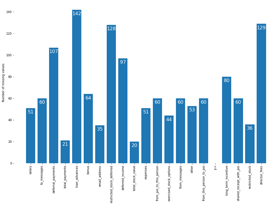
The most common missing values are loan_advances and director_fees, which are probably zero for most employees. Because the spreadsheet uses NaN to mean “not paid”, we will replace all missing values with 0 to make the data easier to analyze.
df = df.fillna(0)
df.head()
| salary | to_messages | deferral_payments | total_payments | loan_advances | bonus | email_address | restricted_stock_deferred | deferred_income | total_stock_value | expenses | from_poi_to_this_person | exercised_stock_options | from_messages | other | from_this_person_to_poi | poi | long_term_incentive | shared_receipt_with_poi | restricted_stock | director_fees | |
|---|---|---|---|---|---|---|---|---|---|---|---|---|---|---|---|---|---|---|---|---|---|
| METTS MARK | 365,788 | 807 | 0 | 1,061,827 | 0 | 600,000 | mark.metts@enron.com | 0 | 0 | 585,062 | 94,299 | 38 | 0 | 29 | 1,740 | 1 | False | 0 | 702 | 585,062 | 0 |
| BAXTER JOHN C | 267,102 | 0 | 1,295,738 | 5,634,343 | 0 | 1,200,000 | 0 | 0 | -1,386,055 | 10,623,258 | 11,200 | 0 | 6,680,544 | 0 | 2,660,303 | 0 | False | 1,586,055 | 0 | 3,942,714 | 0 |
| ELLIOTT STEVEN | 170,941 | 0 | 0 | 211,725 | 0 | 350,000 | steven.elliott@enron.com | 0 | -400,729 | 6,678,735 | 78,552 | 0 | 4,890,344 | 0 | 12,961 | 0 | False | 0 | 0 | 1,788,391 | 0 |
| CORDES WILLIAM R | 0 | 764 | 0 | 0 | 0 | 0 | bill.cordes@enron.com | 0 | 0 | 1,038,185 | 0 | 10 | 651,850 | 12 | 0 | 0 | False | 0 | 58 | 386,335 | 0 |
| HANNON KEVIN P | 243,293 | 1,045 | 0 | 288,682 | 0 | 1,500,000 | kevin.hannon@enron.com | 0 | -3,117,011 | 6,391,065 | 34,039 | 32 | 5,538,001 | 32 | 11,350 | 21 | True | 1,617,011 | 1,035 | 853,064 | 0 |
Let’s look at the checksum values to make sure everything checks out. By “checksums”, I’m referring to values that are supposed to be the sum of other values in the table. They can be used to find errors in the data quickly. In this case, the total_payments field is supposed to be the sum of all the payment categories: salary, bonus, long_term_incentive, deferred_income, deferral_payments, loan_advances, other, expenses, and director_fees.
The original spreadsheet divides up the information into payments and stock value. We’ll do that now and add a separate category for the email.
payment_categories = [
    "salary",
    "bonus",
    "long_term_incentive",
    "deferred_income",
    "deferral_payments",
    "loan_advances",
    "other",
    "expenses",
    "director_fees",
    "total_payments",
]
stock_value_categories = [
    "exercised_stock_options",
    "restricted_stock",
    "restricted_stock_deferred",
    "total_stock_value",
]
Now let’s sum together all the payment categories (except total_payments) and compare it to the total payments. It should be the same value. We’ll print out any rows that aren’t the same.
# Look at the instances where the total we calculate is not equal to the total listed on the spreadsheet
df[df[payment_categories[:-1]].sum(axis="columns") != df["total_payments"]][payment_categories]
| salary | bonus | long_term_incentive | deferred_income | deferral_payments | loan_advances | other | expenses | director_fees | total_payments | |
|---|---|---|---|---|---|---|---|---|---|---|
| BELFER ROBERT | 0 | 0 | 0 | 0 | -102,500 | 0 | 0 | 0 | 3,285 | 102,500 |
| BHATNAGAR SANJAY | 0 | 0 | 0 | 0 | 0 | 0 | 137,864 | 0 | 137,864 | 15,456,290 |
df[df[stock_value_categories[:-1]].sum(axis="columns") != df["total_stock_value"]][stock_value_categories]
| exercised_stock_options | restricted_stock | restricted_stock_deferred | total_stock_value | |
|---|---|---|---|---|
| BELFER ROBERT | 3,285 | 0 | 44,093 | -44,093 |
| BHATNAGAR SANJAY | 2,604,490 | -2,604,490 | 15,456,290 | 0 |
On the original spreadsheet, 102,500 is listed in Robert Belfer’s deferred income section, not in deferral payments. And 3,285 should be the expenses column, director fees should be 102,500, and total payments should be 3,285. It looks like everything shifted one column to the right. We’ll have to move it one to the left to fix it. The opposite happened to Sanjay Bhatnagar, so we’ll have to move his columns to the right to fix them. Let’s do that now.
df.loc["BELFER ROBERT"]
salary                               0
to_messages                          0
deferral_payments             -102,500
total_payments                 102,500
loan_advances                        0
bonus                                0
email_address                        0
restricted_stock_deferred       44,093
deferred_income                      0
total_stock_value              -44,093
expenses                             0
from_poi_to_this_person              0
exercised_stock_options          3,285
from_messages                        0
other                                0
from_this_person_to_poi              0
poi                              False
long_term_incentive                  0
shared_receipt_with_poi              0
restricted_stock                     0
director_fees                    3,285
Name: BELFER ROBERT, dtype: object
Unfortunately, the order of the columns in the actual spreadsheet is different than the one in this dataset, so I can’t use pop to push them all over one. I’ll have to manually fix every incorrect value.
df.loc[("BELFER ROBERT", "deferral_payments")] = 0
df.loc[("BELFER ROBERT", "total_payments")] = 3285
df.loc[("BELFER ROBERT", "restricted_stock_deferred")] = -44093
df.loc[("BELFER ROBERT", "deferred_income")] = -102500
df.loc[("BELFER ROBERT", "total_stock_value")] = 0
df.loc[("BELFER ROBERT", "expenses")] = 3285
df.loc[("BELFER ROBERT", "exercised_stock_options")] = 0
df.loc[("BELFER ROBERT", "restricted_stock")] = 44093
df.loc[("BELFER ROBERT", "director_fees")] = 102500
df.loc["BHATNAGAR SANJAY"]
salary                                                0
to_messages                                         523
deferral_payments                                     0
total_payments                               15,456,290
loan_advances                                         0
bonus                                                 0
email_address                sanjay.bhatnagar@enron.com
restricted_stock_deferred                    15,456,290
deferred_income                                       0
total_stock_value                                     0
expenses                                              0
from_poi_to_this_person                               0
exercised_stock_options                       2,604,490
from_messages                                        29
other                                           137,864
from_this_person_to_poi                               1
poi                                               False
long_term_incentive                                   0
shared_receipt_with_poi                             463
restricted_stock                             -2,604,490
director_fees                                   137,864
Name: BHATNAGAR SANJAY, dtype: object
df.loc[("BHATNAGAR SANJAY", "total_payments")] = 137864
df.loc[("BHATNAGAR SANJAY", "restricted_stock_deferred")] = -2604490
df.loc[("BHATNAGAR SANJAY", "total_stock_value")] = 15456290
df.loc[("BHATNAGAR SANJAY", "expenses")] = 137864
df.loc[("BHATNAGAR SANJAY", "exercised_stock_options")] = 15456290
df.loc[("BHATNAGAR SANJAY", "other")] = 0
df.loc[("BHATNAGAR SANJAY", "restricted_stock")] = 2604490
df.loc[("BHATNAGAR SANJAY", "director_fees")] = 0
Let’s check to make sure that fixes our problems.
print(df[df[payment_categories[:-1]].sum(axis="columns") != df["total_payments"]][payment_categories])
print(df[df[stock_value_categories[:-1]].sum(axis="columns") != df["total_stock_value"]][stock_value_categories])
Empty DataFrame
Columns: [salary, bonus, long_term_incentive, deferred_income, deferral_payments, loan_advances, other, expenses, director_fees, total_payments]
Index: []
Empty DataFrame
Columns: [exercised_stock_options, restricted_stock, restricted_stock_deferred, total_stock_value]
Index: []
Looks good!
Look for Anomalies in the Data
Now we’re going to use a couple of functions provided by the Udacity class. They help to get data out of the dictionaries and into a more usable form. Here they are:
def featureFormat(
    dictionary, features, remove_NaN=True, remove_all_zeroes=True, remove_any_zeroes=False, sort_keys=False
):
    """ convert dictionary to numpy array of features
        remove_NaN = True will convert "NaN" string to 0.0
        remove_all_zeroes = True will omit any data points for which
            all the features you seek are 0.0
        remove_any_zeroes = True will omit any data points for which
            any of the features you seek are 0.0
        sort_keys = True sorts keys by alphabetical order. Setting the value as
            a string opens the corresponding pickle file with a preset key
            order (this is used for Python 3 compatibility, and sort_keys
            should be left as False for the course mini-projects).
        NOTE: first feature is assumed to be 'poi' and is not checked for
            removal for zero or missing values.
    """

    return_list = []

    # Key order - first branch is for Python 3 compatibility on mini-projects,
    # second branch is for compatibility on final project.
    if isinstance(sort_keys, str):
        import pickle

        keys = pickle.load(open(sort_keys, "rb"))
    elif sort_keys:
        keys = sorted(dictionary.keys())
    else:
        keys = list(dictionary.keys())

    for key in keys:
        tmp_list = []
        for feature in features:
            try:
                dictionary[key][feature]
            except KeyError:
                print("error: key ", feature, " not present")
                return
            value = dictionary[key][feature]
            if value == "NaN" and remove_NaN:
                value = 0
            tmp_list.append(float(value))

        # Logic for deciding whether or not to add the data point.
        append = True
        # exclude 'poi' class as criteria.
        if features[0] == "poi":
            test_list = tmp_list[1:]
        else:
            test_list = tmp_list
        ### if all features are zero and you want to remove
        ### data points that are all zero, do that here
        if remove_all_zeroes:
            append = False
            for item in test_list:
                if item != 0 and item != "NaN":
                    append = True
                    break
        ### if any features for a given data point are zero
        ### and you want to remove data points with any zeroes,
        ### handle that here
        if remove_any_zeroes:
            if 0 in test_list or "NaN" in test_list:
                append = False
        ### Append the data point if flagged for addition.
        if append:
            return_list.append(np.array(tmp_list))

    return np.array(return_list)


def targetFeatureSplit(data):
    """
        given a numpy array like the one returned from
        featureFormat, separate out the first feature
        and put it into its own list (this should be the
        quantity you want to predict)

        return targets and features as separate lists

        (sklearn can generally handle both lists and numpy arrays as
        input formats when training/predicting)
    """

    target = []
    features = []
    for item in data:
        target.append(item[0])
        features.append(item[1:])

    return target, features
One of the best ways to detect anomalies is to graph the data. Anomalies often stick out in these graphs. Let’s take a look at how salary correlates with bonus. I suspect it will be positive and fairly strong.
### read in data dictionary, convert to numpy array

features = ["salary", "bonus"]
data = featureFormat(enron_data, features)

for point in data:
    salary = point[0]
    bonus = point[1]
    plt.scatter(salary, bonus)

plt.xlabel("salary")
plt.ylabel("bonus")
plt.show()
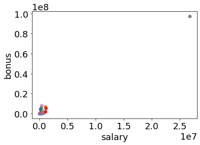
OK, someone’s bonus and salary are way higher than everyone else’s. That looks suspicious so let’s take a look at it.
df[df["salary"] > 10000000]
| salary | to_messages | deferral_payments | total_payments | loan_advances | bonus | email_address | restricted_stock_deferred | deferred_income | total_stock_value | expenses | from_poi_to_this_person | exercised_stock_options | from_messages | other | from_this_person_to_poi | poi | long_term_incentive | shared_receipt_with_poi | restricted_stock | director_fees | |
|---|---|---|---|---|---|---|---|---|---|---|---|---|---|---|---|---|---|---|---|---|---|
| TOTAL | 26,704,229 | 0 | 32,083,396 | 309,886,585 | 83,925,000 | 97,343,619 | 0 | -7,576,788 | -27,992,891 | 434,509,511 | 5,235,198 | 0 | 311,764,000 | 0 | 42,667,589 | 0 | False | 48,521,928 | 0 | 130,322,299 | 1,398,517 |
Ah, there’s an “employee” named “TOTAL” in the spreadsheet. Having a row that is the total of our other rows will mess up our statistics, so we’ll remove it. We’ll also remove The Travel Agency in the Park that we noticed earlier.
entries_to_delete = ["THE TRAVEL AGENCY IN THE PARK", "TOTAL"]
for entry in entries_to_delete:
    if entry in df.index:
        df = df.drop(entry)
Now let’s look again.
### read in data dictionary, convert to numpy array

features = ["salary", "bonus"]
# data = df[["salary", "bonus"]]

salary = df["salary"].values / 1000
bonus = df["bonus"].values / 1000
plt.scatter(salary, bonus)

plt.xlabel("Salary (thousands of dollars)")
plt.ylabel("Bonus (thousands of dollars)")
plt.show()
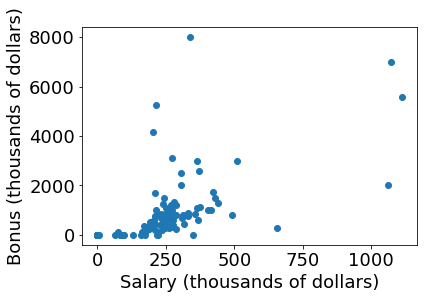
That looks better.
Now that we’ve cleaned up the data let’s save it as a CSV so we can pick it up and do some analysis on it another time.
clean_file = "clean_df.csv"
df.to_csv(path + clean_file, index_label="name")