
Many robot arms use 6 or 7 actuators to control where the hand ends up. This might seem like overkill for positioning a hand in 3D space, but in this post I want to dig into the math behind how robot arms work.
Let’s say we have 7 actuators. We know that the relationship between joint angles $\boldsymbol{\theta} \in \mathbb{R}^7$ and hand position $\mathbf{p} \in \mathbb{R}^3$ is given by some function: \(\mathbf{p} = f(\boldsymbol{\theta})\)
What we need to know is, if I move this actuator a tiny bit, what happens to the hand. That is, what can help us convert a tiny change in a joint angle to a change in the hand position.
\[\Delta \mathbf{p} = ? \cdot \Delta \boldsymbol{\theta}\]The answer is our old friend the Jacobian. The Jacobian is essentially the multivariable generalization of a derivative. The Jacobian $J$ is (in this case) a $3 \times 7$ matrix that tells us exactly what we’re looking for: “If I wiggle each joint a little, how does the hand move?”
\[\Delta \mathbf{p} = J \cdot \Delta \boldsymbol{\theta}\]Simple 2D Robot Hand
However, we’re going to simplify a bit. Let’s think of a robot hand that can only move in two dimensions and has three actuators.
import numpy as np
import matplotlib.pyplot as plt
from scipy.linalg import null_space

np.random.seed(42)
plt.style.use('seaborn-v0_8-whitegrid')
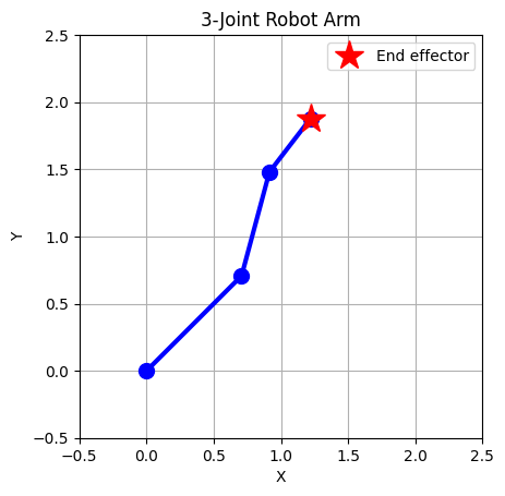
Let’s say the robot arm has the following lengths and are at the following angles:
# 3-joint arm
link_lengths = [1.0, 0.8, 0.5]
theta = np.array([np.pi/4, np.pi/6, -np.pi/8])
Now we can compute the full position of each link.
def forward_kinematics_2d(theta, link_lengths):
    """Compute end effector position given joint angles."""
    positions = [(0, 0)]  # base at origin

    cumulative_angle = 0
    x, y = 0, 0

    for length, angle in zip(link_lengths, theta):
        cumulative_angle += angle
        x += length * np.cos(cumulative_angle)
        y += length * np.sin(cumulative_angle)
        positions.append((x, y))

    positions = np.array(positions)

    return positions
positions = forward_kinematics_2d(theta, link_lengths)
Let’s plot those to see what we’ve got.
plt.plot(positions[:, 0], positions[:, 1], 'bo-', linewidth=3, markersize=10)
plt.plot(positions[-1, 0], positions[-1, 1], 'r*', markersize=20, label='End effector')
plt.xlim(-0.5, 2.5)
plt.ylim(-0.5, 2.5)
plt.gca().set_aspect('equal')
plt.xlabel('X')
plt.ylabel('Y')
plt.title('3-Joint Robot Arm')
plt.legend()
plt.grid(True)
OK, now let’s compute the Jacobian. All we need to know is the section lengths and angles, which we have.
print(link_lengths)
print(theta)
[1.0, 0.8, 0.5]
[ 0.78539816  0.52359878 -0.39269908]
def jacobian_2d(theta, link_lengths):
    """Compute Jacobian for 2D robot arm."""
    n = len(theta)
    J = np.zeros((2, n))  # 2 because the hand moves in two dimensions

    for i in range(n):
        # Rotating joint i affects all links from i onward
        for j in range(i, n):
            angle_j = sum(theta[:j+1])
            J[0, i] += -link_lengths[j] * np.sin(angle_j)
            J[1, i] += link_lengths[j] * np.cos(angle_j)

    return J
J = jacobian_2d(theta, link_lengths)
J
array([[-1.87652411, -1.16941733, -0.39667667],
       [ 1.21854273,  0.51143595,  0.30438071]])
Now we can visualize the Jacobian.
# Show Jacobian
plt.figure(figsize=(7, 4))
im = plt.imshow(J, cmap='RdBu', aspect='auto')
plt.xticks([0, 1, 2], ['Joint 1', 'Joint 2', 'Joint 3'])
plt.yticks([0, 1], ['X movement', 'Y movement'])
plt.title('Jacobian Matrix (2×3)\nHow each joint affects end position')
plt.colorbar(im)

# Add values
for i in range(2):
    for j in range(3):
        plt.text(j, i, f'{J[i,j]:.2f}', ha='center', va='center', fontsize=12)

plt.tight_layout()
plt.show()
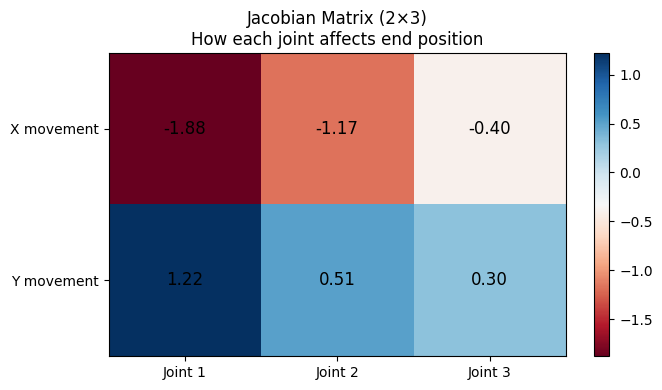
This tells us that if we move joint 1, it will cause a Y movement of 1.22 and an X movement of -1.88. We can also see that moving the first joint has the largest effect, and moving the last has the least, which is what we would intuitively expect.
How to Move and Keep Your Hand Still
In this case, we know that the rank is at most 2 because each column is a vector in \(\mathbb{R}^2\) (it has 2 entries). You can never have more than 2 linearly independent vectors in $\mathbb{R}^2$. (So, as a general rule, rank(A) ≤ min(rows, columns))
And we know from the rank-nullity theorem that the number of columns of a matrix is the sum of the rank and nullity of that matrix.
As a reminder, for a matrix A with n columns: rank(A) + nullity(A) = n
Or in words: (dimensions of output space you actually hit) + (dimensions that get crushed to zero) = (dimensions you started with)
So the nullity in this case is at least 1 (that’s \(3 - 2 = 1\)).
We can use numpy to compute the rank and scipy to find the null space. The null space is the set of all joint movements that don’t move the hand at all. If you want to think about this intuitively, think about how you can put your finger on something in front of you but still wiggle your arm without moving your finger. Those movements are in the null space.
# Compute rank and null space
rank = np.linalg.matrix_rank(J)
ns = null_space(J)
nullity = ns.shape[1]
print(f"2D arm: 3 joints → 2D position")
print(f"Jacobian shape: {J.shape}")
print(f"Rank: {rank}")
print(f"Nullity: {nullity}")
2D arm: 3 joints → 2D position
Jacobian shape: (2, 3)
Rank: 2
Nullity: 1
We also have a direction in joint space we can move along without affecting the hand position:
print(f"Null space: {ns.flatten().round(3)}")
Null space: [-0.308 0.176 0.935]
Let’s show that we can move some amount in that direction without moving the hand.
fig, ax = plt.subplots(figsize=(10, 8))

colors = plt.cm.viridis(np.linspace(0, 1, 7))

# Move along null space direction
for i, alpha in enumerate(np.linspace(-0.3, 0.3, 7)):
    theta_new = theta + alpha * ns.flatten()
    positions = forward_kinematics_2d(theta_new, link_lengths)
    positions = np.array(positions)

    ax.plot(positions[:, 0], positions[:, 1], 'o-', color=colors[i],
            linewidth=2, markersize=8, alpha=0.7, label=f'α={alpha:.2f}')

# Mark end effector (should be same for all!)
ax.plot(positions[-1, 0], positions[-1, 1], 'r*', markersize=25,
        label='End effector (same!)', zorder=10)

ax.set_xlim(-0.5, 2.5)
ax.set_ylim(-0.5, 2.5)
ax.set_aspect('equal')
ax.set_xlabel('X')
ax.set_ylabel('Y')
ax.set_title('Null Space Motion: Joints Move, Hand Stays Still\n(Different configurations, same end position)')
ax.legend(loc='upper left')
ax.grid(True)

plt.show()
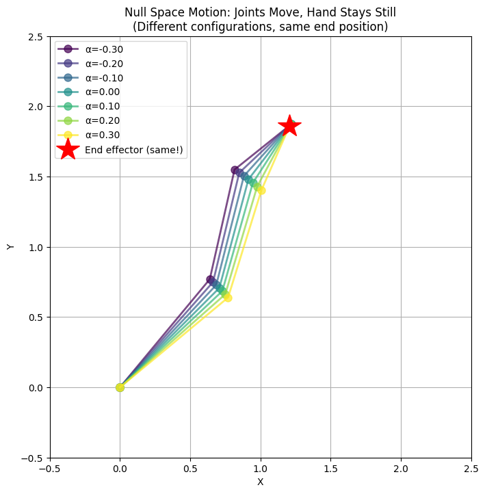
A note on linearization: The Jacobian gives us a local linear approximation. For small movements along the null space, the hand stays almost perfectly still. But for larger movements, you’ll notice slight drift because the true relationship $\mathbf{p} = f(\boldsymbol{\theta})$ is nonlinear. The Jacobian is only exact in the limit of infinitesimal movements.
Why Redundancy Matters
So why do robots have these “extra” degrees of freedom? The null space isn’t wasted—it’s incredibly useful:
- Obstacle avoidance: You can move your elbow out of the way without moving your hand
- Joint limit avoidance: If one joint is near its limit, you can use null space motion to redistribute the load to other joints
- Optimizing secondary objectives: While your hand stays on target, you can minimize energy consumption, maximize manipulability, or maintain a comfortable posture
- Singularity avoidance: The null space can help you steer away from configurations where control becomes difficult (more on this below)
Think about reaching for something on a shelf. Your hand might stay in place while you adjust your elbow and shoulder to find a comfortable position. That’s null space motion in action.
Scaling Up
OK, let’s think about how this would work with our 7-joint robot arm controlling a hand in 3D space. Now, the Jacobian is \(3 \times 7\).
This time, we know that the rank is at most 3 because each column is a vector in \(\mathbb{R}^3\) (it has 3 entries). Again, you can never have more than 3 linearly independent vectors in \(\mathbb{R}^3\).
And we use the rank-nullity theorem to show that the nullity is at least 4 (that’s \(7 - 3 = 4\)). With a nullity of at least 4, we have at least 4 dimensions of freedom to move the joints while keeping the hand perfectly still.
But wait—what about orientation? In practice, robots often need to control not just where the hand is, but how it’s oriented (think of a robot pouring a cup of coffee—the angle matters!). Position requires 3 DOF, and orientation requires 3 more (roll, pitch, yaw), for a total of 6 DOF. This is why 6-joint robot arms are so common—they have exactly the right number of joints to achieve any position and orientation in their workspace (with rank 6 and nullity 0).
A 7-joint arm controlling position and orientation has a \(6 \times 7\) Jacobian with nullity 1. That single extra degree of freedom gives you the flexibility to do things like keep your elbow away from obstacles while maintaining full control of the end effector.
A Word on Singularities
Everything we’ve discussed assumes the Jacobian has full rank. But what happens when it doesn’t?
When a robot arm is fully extended (or fully folded), some columns of the Jacobian become linearly dependent, and the rank drops. These configurations are called singularities. At a singularity:
- The null space grows—there are more ways to move without affecting the hand (or, equivalently, certain hand movements become impossible)
- Small movements in task space may require huge joint velocities
- Control becomes numerically unstable
Think of your arm fully extended in front of you. Try to move your hand directly backward toward your shoulder—you can’t do it smoothly without bending your elbow first. That’s a singularity.
Robot controllers actively avoid singularities, often by using the null space freedom (when available) to steer away from these problematic configurations.
So why do robot arms have 6 or 7 joints? Six joints give you full control over position and orientation with no redundancy. Seven joints add one degree of null space freedom, letting the robot optimize secondary objectives (like avoiding obstacles or joint limits) while still hitting the target.