In this post, let’s visualize the internals of a transformer model. These visualizations reveal some interesting patterns that can help us understand how well the training is going.

We’ll be looking at GPT-2 small (125M parameters). When analyzing transformer weights, there are several patterns we typically look for:

• Periodic patterns in positional embeddings that show how the model encodes position information
• Gaussian-like distributions in attention weights, which suggest good initialization and training
• Specialized attention heads that may focus on different aspects of the input
• Layer-wise progression showing increasing specialization in deeper layers
• Clustering patterns among attention heads that might indicate functional grouping

These patterns matter because they can help us understand if a model is well-trained and how it processes information. Unusual patterns might indicate training issues or interesting specializations we can leverage.

Table of Contents

• Overall Model Architecture
• Positional Embeddings
  • Correlation Between Positions
• Attention Weights
  • Layer-by-Layer Evolution
• Attention Head Patterns
• Conclusion

import warnings

import numpy as np
import seaborn as sns
import torch
from matplotlib import pyplot as plt
from scipy import stats
from scipy.cluster.hierarchy import dendrogram, linkage
from scipy.stats import pearsonr, zscore
from sklearn.decomposition import PCA
from sklearn.preprocessing import StandardScaler
from transformers import GPT2LMHeadModel

warnings.filterwarnings('ignore')

We’ll use the transformers library to get a trained GPT2 model.

model = GPT2LMHeadModel.from_pretrained('gpt2')
state_dict = model.state_dict()

Overall Model Architecture

First, let’s look at the basic model architecture.

def analyze_model_architecture():
    layer_info = []
    total_params = 0
    
    for k, v in state_dict.items():
        num_params = np.prod(v.shape)
        total_params += num_params
        
        # Categorize the layer
        if 'wpe' in k:
            category = 'Positional Embedding'
        elif 'wte' in k:
            category = 'Token Embedding'
        elif 'attn' in k:
            category = 'Attention'
        elif 'mlp' in k:
            category = 'Feed Forward'
        elif 'ln' in k:
            category = 'Layer Norm'
        else:
            category = 'Other'
            
        # Extract layer number if present
        layer_num = None
        if 'h.' in k:
            layer_num = int(k.split('.')[2])
            
        layer_info.append({
            'name': k,
            'shape': v.shape,
            'params': num_params,
            'category': category,
            'layer': layer_num,
            'size_mb': num_params * 4 / (1024 * 1024)  # Assuming float32
        })
    
    return layer_info, total_params

def visualize_architecture(layer_info, total_params):
    # 1. Parameter distribution by category
    plt.figure(figsize=(12, 6))
    category_params = {}
    for layer in layer_info:
        category_params[layer['category']] = category_params.get(layer['category'], 0) + layer['params']
    
    categories = list(category_params.keys())
    params = list(category_params.values())
    
    plt.pie(params, labels=categories, autopct='%1.1f%%')
    plt.title('Distribution of Parameters by Category')
    plt.close()
    
    # 2. Layer sizes across model depth
    plt.figure(figsize=(15, 6))
    layer_sizes = []
    layer_numbers = []
    layer_categories = []
    
    for info in layer_info:
        if info['layer'] is not None:
            layer_sizes.append(info['size_mb'])
            layer_numbers.append(info['layer'])
            layer_categories.append(info['category'])
    
    scatter = plt.scatter(layer_numbers, layer_sizes, c=[hash(cat) for cat in layer_categories], 
                         alpha=0.6, s=100)
    plt.xlabel('Layer Number')
    plt.ylabel('Size (MB)')
    plt.title('Layer Sizes Across Model Depth')
    plt.grid(True, alpha=0.3)
    plt.close()
    
    # Return formatted string of architecture summary
    summary = "GPT-2 Architecture Summary\n"
    summary += "========================\n\n"
    summary += f"Total Parameters: {total_params:,} ({total_params * 4 / (1024 * 1024):.2f} MB)\n\n"
    
    # Group by category
    category_layers = {}
    for layer in layer_info:
        if layer['category'] not in category_layers:
            category_layers[layer['category']] = []
        category_layers[layer['category']].append(layer)
    
    for category, layers in category_layers.items():
        summary += f"\n{category}\n{'-' * len(category)}\n"
        for layer in layers:
            shape_str = ' × '.join(str(x) for x in layer['shape'])
            summary += f"{layer['name']}: {shape_str} ({layer['params']:,} params)\n"
            
    return summary

layer_info, total_params = analyze_model_architecture()
summary = visualize_architecture(layer_info, total_params)
print(summary)

GPT-2 Architecture Summary
========================

Total Parameters: 163,037,184 (621.94 MB)


Token Embedding
---------------
transformer.wte.weight: 50257 × 768 (38,597,376 params)

Positional Embedding
--------------------
transformer.wpe.weight: 1024 × 768 (786,432 params)

Layer Norm
----------
transformer.h.0.ln_1.weight: 768 (768 params)
transformer.h.0.ln_1.bias: 768 (768 params)
transformer.h.0.ln_2.weight: 768 (768 params)
transformer.h.0.ln_2.bias: 768 (768 params)
transformer.h.1.ln_1.weight: 768 (768 params)
transformer.h.1.ln_1.bias: 768 (768 params)
transformer.h.1.ln_2.weight: 768 (768 params)
transformer.h.1.ln_2.bias: 768 (768 params)
transformer.h.2.ln_1.weight: 768 (768 params)
transformer.h.2.ln_1.bias: 768 (768 params)
transformer.h.2.ln_2.weight: 768 (768 params)
transformer.h.2.ln_2.bias: 768 (768 params)
transformer.h.3.ln_1.weight: 768 (768 params)
transformer.h.3.ln_1.bias: 768 (768 params)
transformer.h.3.ln_2.weight: 768 (768 params)
transformer.h.3.ln_2.bias: 768 (768 params)
transformer.h.4.ln_1.weight: 768 (768 params)
transformer.h.4.ln_1.bias: 768 (768 params)
transformer.h.4.ln_2.weight: 768 (768 params)
transformer.h.4.ln_2.bias: 768 (768 params)
transformer.h.5.ln_1.weight: 768 (768 params)
transformer.h.5.ln_1.bias: 768 (768 params)
transformer.h.5.ln_2.weight: 768 (768 params)
transformer.h.5.ln_2.bias: 768 (768 params)
transformer.h.6.ln_1.weight: 768 (768 params)
transformer.h.6.ln_1.bias: 768 (768 params)
transformer.h.6.ln_2.weight: 768 (768 params)
transformer.h.6.ln_2.bias: 768 (768 params)
transformer.h.7.ln_1.weight: 768 (768 params)
transformer.h.7.ln_1.bias: 768 (768 params)
transformer.h.7.ln_2.weight: 768 (768 params)
transformer.h.7.ln_2.bias: 768 (768 params)
transformer.h.8.ln_1.weight: 768 (768 params)
transformer.h.8.ln_1.bias: 768 (768 params)
transformer.h.8.ln_2.weight: 768 (768 params)
transformer.h.8.ln_2.bias: 768 (768 params)
transformer.h.9.ln_1.weight: 768 (768 params)
transformer.h.9.ln_1.bias: 768 (768 params)
transformer.h.9.ln_2.weight: 768 (768 params)
transformer.h.9.ln_2.bias: 768 (768 params)
transformer.h.10.ln_1.weight: 768 (768 params)
transformer.h.10.ln_1.bias: 768 (768 params)
transformer.h.10.ln_2.weight: 768 (768 params)
transformer.h.10.ln_2.bias: 768 (768 params)
transformer.h.11.ln_1.weight: 768 (768 params)
transformer.h.11.ln_1.bias: 768 (768 params)
transformer.h.11.ln_2.weight: 768 (768 params)
transformer.h.11.ln_2.bias: 768 (768 params)
transformer.ln_f.weight: 768 (768 params)
transformer.ln_f.bias: 768 (768 params)

Attention
---------
transformer.h.0.attn.c_attn.weight: 768 × 2304 (1,769,472 params)
transformer.h.0.attn.c_attn.bias: 2304 (2,304 params)
transformer.h.0.attn.c_proj.weight: 768 × 768 (589,824 params)
transformer.h.0.attn.c_proj.bias: 768 (768 params)
transformer.h.1.attn.c_attn.weight: 768 × 2304 (1,769,472 params)
transformer.h.1.attn.c_attn.bias: 2304 (2,304 params)
transformer.h.1.attn.c_proj.weight: 768 × 768 (589,824 params)
transformer.h.1.attn.c_proj.bias: 768 (768 params)
transformer.h.2.attn.c_attn.weight: 768 × 2304 (1,769,472 params)
transformer.h.2.attn.c_attn.bias: 2304 (2,304 params)
transformer.h.2.attn.c_proj.weight: 768 × 768 (589,824 params)
transformer.h.2.attn.c_proj.bias: 768 (768 params)
transformer.h.3.attn.c_attn.weight: 768 × 2304 (1,769,472 params)
transformer.h.3.attn.c_attn.bias: 2304 (2,304 params)
transformer.h.3.attn.c_proj.weight: 768 × 768 (589,824 params)
transformer.h.3.attn.c_proj.bias: 768 (768 params)
transformer.h.4.attn.c_attn.weight: 768 × 2304 (1,769,472 params)
transformer.h.4.attn.c_attn.bias: 2304 (2,304 params)
transformer.h.4.attn.c_proj.weight: 768 × 768 (589,824 params)
transformer.h.4.attn.c_proj.bias: 768 (768 params)
transformer.h.5.attn.c_attn.weight: 768 × 2304 (1,769,472 params)
transformer.h.5.attn.c_attn.bias: 2304 (2,304 params)
transformer.h.5.attn.c_proj.weight: 768 × 768 (589,824 params)
transformer.h.5.attn.c_proj.bias: 768 (768 params)
transformer.h.6.attn.c_attn.weight: 768 × 2304 (1,769,472 params)
transformer.h.6.attn.c_attn.bias: 2304 (2,304 params)
transformer.h.6.attn.c_proj.weight: 768 × 768 (589,824 params)
transformer.h.6.attn.c_proj.bias: 768 (768 params)
transformer.h.7.attn.c_attn.weight: 768 × 2304 (1,769,472 params)
transformer.h.7.attn.c_attn.bias: 2304 (2,304 params)
transformer.h.7.attn.c_proj.weight: 768 × 768 (589,824 params)
transformer.h.7.attn.c_proj.bias: 768 (768 params)
transformer.h.8.attn.c_attn.weight: 768 × 2304 (1,769,472 params)
transformer.h.8.attn.c_attn.bias: 2304 (2,304 params)
transformer.h.8.attn.c_proj.weight: 768 × 768 (589,824 params)
transformer.h.8.attn.c_proj.bias: 768 (768 params)
transformer.h.9.attn.c_attn.weight: 768 × 2304 (1,769,472 params)
transformer.h.9.attn.c_attn.bias: 2304 (2,304 params)
transformer.h.9.attn.c_proj.weight: 768 × 768 (589,824 params)
transformer.h.9.attn.c_proj.bias: 768 (768 params)
transformer.h.10.attn.c_attn.weight: 768 × 2304 (1,769,472 params)
transformer.h.10.attn.c_attn.bias: 2304 (2,304 params)
transformer.h.10.attn.c_proj.weight: 768 × 768 (589,824 params)
transformer.h.10.attn.c_proj.bias: 768 (768 params)
transformer.h.11.attn.c_attn.weight: 768 × 2304 (1,769,472 params)
transformer.h.11.attn.c_attn.bias: 2304 (2,304 params)
transformer.h.11.attn.c_proj.weight: 768 × 768 (589,824 params)
transformer.h.11.attn.c_proj.bias: 768 (768 params)

Feed Forward
------------
transformer.h.0.mlp.c_fc.weight: 768 × 3072 (2,359,296 params)
transformer.h.0.mlp.c_fc.bias: 3072 (3,072 params)
transformer.h.0.mlp.c_proj.weight: 3072 × 768 (2,359,296 params)
transformer.h.0.mlp.c_proj.bias: 768 (768 params)
transformer.h.1.mlp.c_fc.weight: 768 × 3072 (2,359,296 params)
transformer.h.1.mlp.c_fc.bias: 3072 (3,072 params)
transformer.h.1.mlp.c_proj.weight: 3072 × 768 (2,359,296 params)
transformer.h.1.mlp.c_proj.bias: 768 (768 params)
transformer.h.2.mlp.c_fc.weight: 768 × 3072 (2,359,296 params)
transformer.h.2.mlp.c_fc.bias: 3072 (3,072 params)
transformer.h.2.mlp.c_proj.weight: 3072 × 768 (2,359,296 params)
transformer.h.2.mlp.c_proj.bias: 768 (768 params)
transformer.h.3.mlp.c_fc.weight: 768 × 3072 (2,359,296 params)
transformer.h.3.mlp.c_fc.bias: 3072 (3,072 params)
transformer.h.3.mlp.c_proj.weight: 3072 × 768 (2,359,296 params)
transformer.h.3.mlp.c_proj.bias: 768 (768 params)
transformer.h.4.mlp.c_fc.weight: 768 × 3072 (2,359,296 params)
transformer.h.4.mlp.c_fc.bias: 3072 (3,072 params)
transformer.h.4.mlp.c_proj.weight: 3072 × 768 (2,359,296 params)
transformer.h.4.mlp.c_proj.bias: 768 (768 params)
transformer.h.5.mlp.c_fc.weight: 768 × 3072 (2,359,296 params)
transformer.h.5.mlp.c_fc.bias: 3072 (3,072 params)
transformer.h.5.mlp.c_proj.weight: 3072 × 768 (2,359,296 params)
transformer.h.5.mlp.c_proj.bias: 768 (768 params)
transformer.h.6.mlp.c_fc.weight: 768 × 3072 (2,359,296 params)
transformer.h.6.mlp.c_fc.bias: 3072 (3,072 params)
transformer.h.6.mlp.c_proj.weight: 3072 × 768 (2,359,296 params)
transformer.h.6.mlp.c_proj.bias: 768 (768 params)
transformer.h.7.mlp.c_fc.weight: 768 × 3072 (2,359,296 params)
transformer.h.7.mlp.c_fc.bias: 3072 (3,072 params)
transformer.h.7.mlp.c_proj.weight: 3072 × 768 (2,359,296 params)
transformer.h.7.mlp.c_proj.bias: 768 (768 params)
transformer.h.8.mlp.c_fc.weight: 768 × 3072 (2,359,296 params)
transformer.h.8.mlp.c_fc.bias: 3072 (3,072 params)
transformer.h.8.mlp.c_proj.weight: 3072 × 768 (2,359,296 params)
transformer.h.8.mlp.c_proj.bias: 768 (768 params)
transformer.h.9.mlp.c_fc.weight: 768 × 3072 (2,359,296 params)
transformer.h.9.mlp.c_fc.bias: 3072 (3,072 params)
transformer.h.9.mlp.c_proj.weight: 3072 × 768 (2,359,296 params)
transformer.h.9.mlp.c_proj.bias: 768 (768 params)
transformer.h.10.mlp.c_fc.weight: 768 × 3072 (2,359,296 params)
transformer.h.10.mlp.c_fc.bias: 3072 (3,072 params)
transformer.h.10.mlp.c_proj.weight: 3072 × 768 (2,359,296 params)
transformer.h.10.mlp.c_proj.bias: 768 (768 params)
transformer.h.11.mlp.c_fc.weight: 768 × 3072 (2,359,296 params)
transformer.h.11.mlp.c_fc.bias: 3072 (3,072 params)
transformer.h.11.mlp.c_proj.weight: 3072 × 768 (2,359,296 params)
transformer.h.11.mlp.c_proj.bias: 768 (768 params)

Other
-----
lm_head.weight: 50257 × 768 (38,597,376 params)

Positional Embeddings

Let’s start with the positional embeddings, which encode position information for the model. First, let’s look at the complete embedding matrix:

plt.figure(figsize=(12, 8))
pos_embeddings = state_dict['transformer.wpe.weight'].numpy()
plt.imshow(pos_embeddings, cmap='RdBu', aspect='auto')
plt.colorbar(label='Weight Value')
plt.title('Full Positional Embeddings Matrix')
plt.xlabel('Embedding Dimension')
plt.ylabel('Position')

Text(0, 0.5, 'Position')

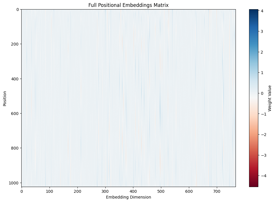
I find it hard to see much in this image (you can also try cmap='grey', but I don’t think it helps much), so instead let’s look at a specific dimension.

plt.figure(figsize=(12, 6))
plt.plot(pos_embeddings[:, 500], linewidth=2)
plt.title('Position Embedding Values (Dimension 500)')
plt.xlabel('Position')
plt.ylabel('Value')
plt.grid(True, alpha=0.3)

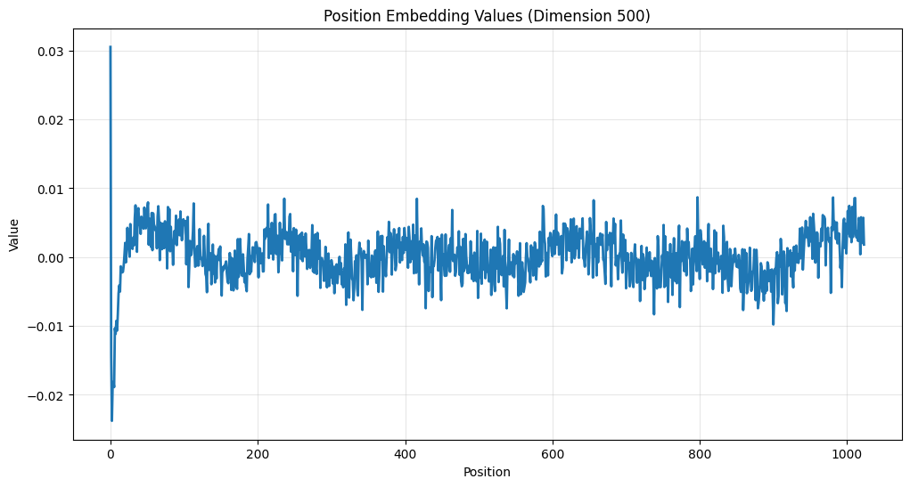
Notice the periodic patterns that emerge - this is not random! These patterns help the model understand relative positions of tokens in the input sequence. You can see the similarity between this and a sine wave. While it used to be common to directly use a sine or cosine wave, now the features are learned, and roughly approximate that shape (other than the very beginning).

Let’s look at a few more.

plt.figure(figsize=(12, 6))
plt.plot(pos_embeddings[:, 400], label='Dimension 400')
plt.plot(pos_embeddings[:, 600], label='Dimension 600')
plt.plot(pos_embeddings[:, 700], label='Dimension 700')
plt.title('Position Embedding Values (Various Dimensions)')
plt.xlabel('Position')
plt.ylabel('Value')
plt.grid(True, alpha=0.3)
plt.legend()

<matplotlib.legend.Legend at 0x13cdaec30>

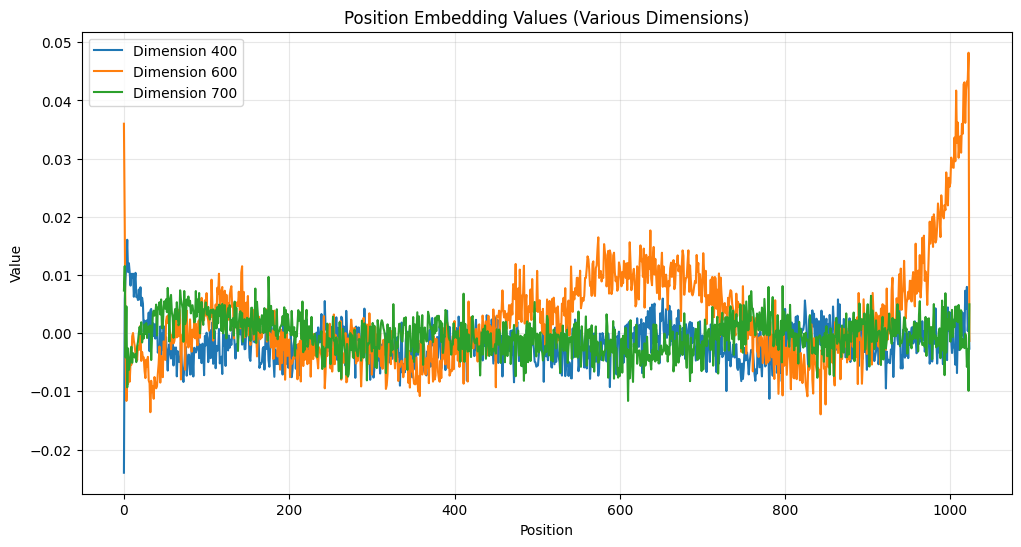
We can also see that some dimensions have high variance and some have low. Take a look at this:

# Choose dimensions based on variance
variances = np.var(pos_embeddings, axis=0)
low_var_dim = np.argmin(variances)
mid_var_dim = len(variances)//2
high_var_dim = np.argmax(variances)

plt.figure(figsize=(12, 6))
plt.plot(pos_embeddings[:, low_var_dim], label=f'Low Variance (dim {low_var_dim})', alpha=0.8)
plt.plot(pos_embeddings[:, mid_var_dim], label=f'Mid Variance (dim {mid_var_dim})', alpha=0.8)
plt.plot(pos_embeddings[:, high_var_dim], label=f'High Variance (dim {high_var_dim})', alpha=0.8)
plt.title('Positional Embeddings: Comparing Dimensions with Different Variances')
plt.xlabel('Position')
plt.ylabel('Value')
plt.legend()
plt.grid(True, alpha=0.3)

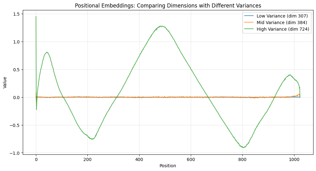
The high variance dimension (724) completely saturates the graph, so you can barely see the mid and low variance dimensions.

Correlation Between Positions

You can also look at the correlation between adjacent positions. I find this very interesting.

# Compute correlation between adjacent positions
correlations = [pearsonr(pos_embeddings[i], pos_embeddings[i+1])[0] 
                for i in range(pos_embeddings.shape[0]-1)]

plt.figure(figsize=(12, 6))
plt.plot(correlations)
plt.title('Correlation Between Adjacent Positions')
plt.xlabel('Position')
plt.ylabel('Correlation with Next Position')
plt.grid(True, alpha=0.3)

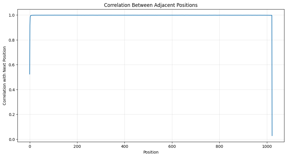
My main takeaway is that there is strong local correlations that indicate smooth transitions between nearby positions.

Attention Weights

There are a lot of ways to analyze the attention weights. Let’s start by looking at the distribution of weights.

# Get weights and calculate statistics
attn_weights = state_dict['transformer.h.0.attn.c_attn.weight'].numpy()
weights_flat = attn_weights.flatten()

# Calculate mean and standard deviation
mu = np.mean(weights_flat)
sigma = np.std(weights_flat)

# Create figure
plt.figure(figsize=(12, 6))

# Plot histogram of actual weights
# Use density=True to make it comparable with the normal distribution
sns.histplot(weights_flat, bins=50, stat='density', label='Actual Weights')

# Create points for normal distribution
x = np.linspace(mu - 4*sigma, mu + 4*sigma, 100)
normal_dist = stats.norm.pdf(x, mu, sigma)

# Plot normal distribution
plt.plot(x, normal_dist, 'r-', lw=2, label=f'Normal Distribution\n(μ={mu:.3f}, σ={sigma:.3f})')

# Add labels and title
plt.title('Distribution of Attention Weights (Layer 0)')
plt.xlabel('Weight Value')
plt.ylabel('Density')
plt.legend()

# Add summary statistics as text
stats_text = f'Skewness: {stats.skew(weights_flat):.3f}\n'
stats_text += f'Kurtosis: {stats.kurtosis(weights_flat):.3f}\n'
stats_text += f'Mean: {mu:.3f}\n'
stats_text += f'Std Dev: {sigma:.3f}'

# Position the text box in the top right
plt.text(0.95, 0.95, stats_text,
         transform=plt.gca().transAxes,
         verticalalignment='top',
         horizontalalignment='right',
         bbox=dict(boxstyle='round', facecolor='white', alpha=0.8))

plt.grid(True, alpha=0.3)
plt.show()

# Print Kolmogorov-Smirnov test results
ks_statistic, p_value = stats.kstest(weights_flat, 'norm', args=(mu, sigma))
print(f"\nKolmogorov-Smirnov test results:")
print(f"KS statistic: {ks_statistic:.4f}")
print(f"p-value: {p_value:.4e}")

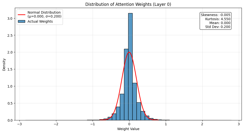
Kolmogorov-Smirnov test results:
KS statistic: 0.0908
p-value: 0.0000e+00

This histogram shows the distribution of attention weights in the first layer. Some observations:

• The distribution is roughly normal but with slightly heavier tails
  • KS statistic of 0.0908, where 0 is a perfect normal distribution and 1 is the opposite, suggests that it’s pretty close to normal
• Most weights are concentrated around zero
• This is common in neural networks - we want weights to be approximately normal but with slightly heavier tails for better learning dynamics

Let’s look at the attention weights more directly. I find that it’s hard to look at them all at once, so it’s better to zoom in to specific parts.

def plot_attention_weights(layer_idx, zoom_ranges=None):
    attn_weights = state_dict[f'transformer.h.{layer_idx}.attn.c_attn.weight'].numpy()
    
    if zoom_ranges is None:
        # Full view
        plt.figure(figsize=(12, 8))
        plt.imshow(attn_weights, cmap='RdBu', aspect='auto')
        plt.colorbar(label='Weight Value')
        plt.title(f'Attention Weights Layer {layer_idx}')
        plt.xlabel('Input Dimension')
        plt.ylabel('Output Dimension')
    else:
        # Zoomed views
        fig, axes = plt.subplots(len(zoom_ranges), 1, figsize=(12, 4*len(zoom_ranges)))
        if len(zoom_ranges) == 1:
            axes = [axes]
        
        for ax, (rows, cols) in zip(axes, zoom_ranges):
            row_start, row_end = rows
            col_start, col_end = cols
            zoomed = attn_weights[row_start:row_end, col_start:col_end]
            im = ax.imshow(zoomed, cmap='RdBu', aspect='auto')
            plt.colorbar(im, ax=ax, label='Weight Value')
            ax.set_title(f'Layer {layer_idx}: Rows {row_start}:{row_end}, Cols {col_start}:{col_end}')
            ax.set_xlabel('Input Dimension')
            ax.set_ylabel('Output Dimension')
        
        plt.tight_layout()

# Plot full and zoomed views for first few layers
zoom_ranges = [
    ((0, 300), (100, 300)),  # Your suggested zoom
    ((300, 600), (200, 400)),  # Another interesting region
]

plot_attention_weights(0)
plot_attention_weights(0, zoom_ranges)

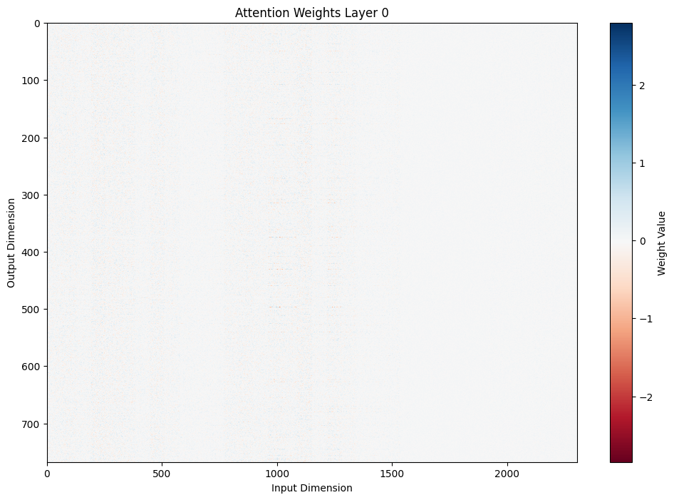
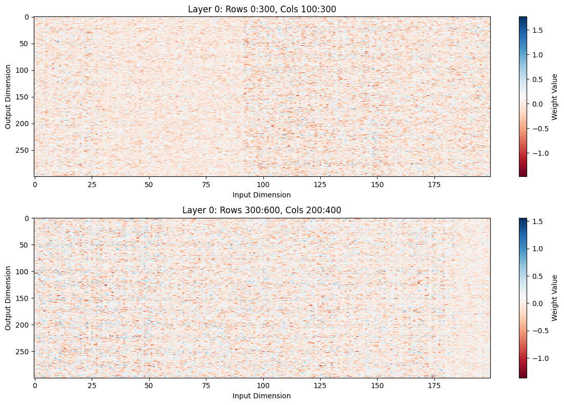
You can tell by zooming in that there’s quite a lot of structure here.

Layer-by-Layer Evolution

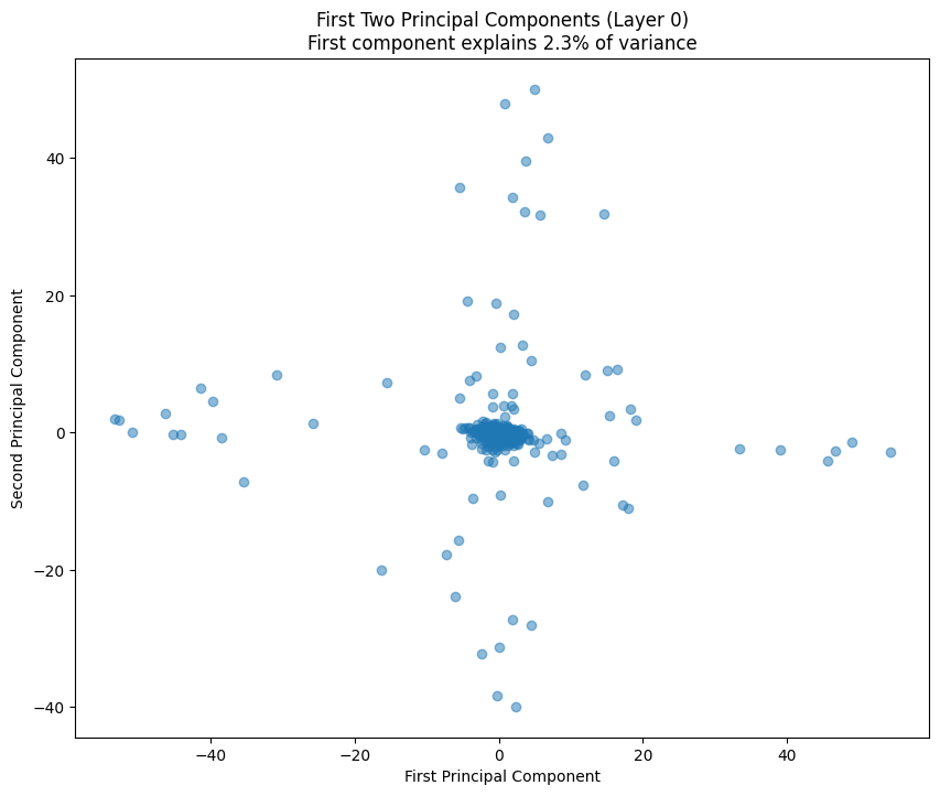
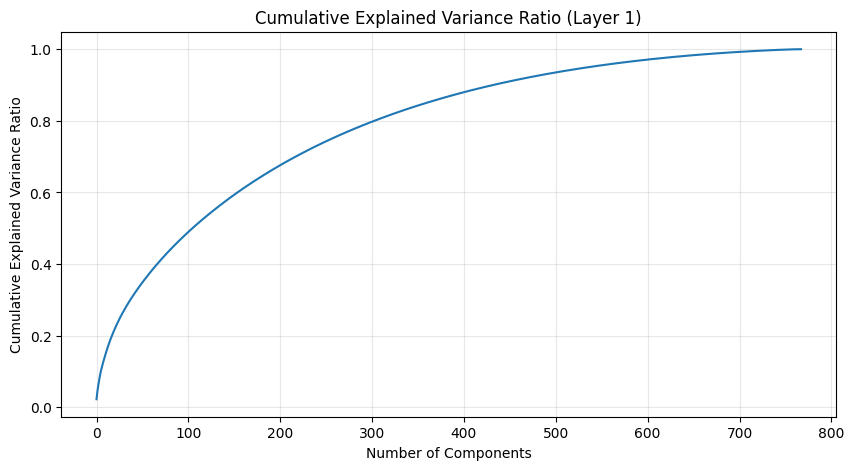
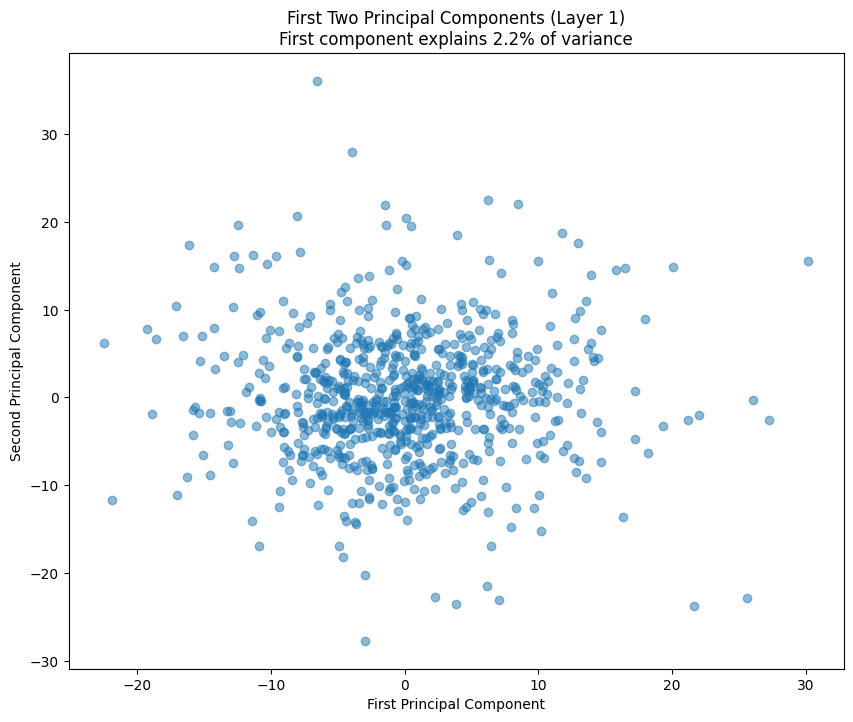
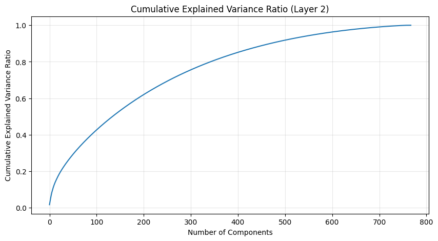
One of the most interesting aspects is how weight patterns change across layers. Let’s start by looking at some PCA of the layers.

def analyze_attention_layer(layer_idx):
    weights = state_dict[f'transformer.h.{layer_idx}.attn.c_attn.weight'].numpy()
    
    # Apply PCA
    pca = PCA()
    scaler = StandardScaler()
    weights_scaled = scaler.fit_transform(weights)
    weights_pca = pca.fit_transform(weights_scaled)
    
    # Plot explained variance ratio
    plt.figure(figsize=(10, 5))
    plt.plot(np.cumsum(pca.explained_variance_ratio_))
    plt.title(f'Cumulative Explained Variance Ratio (Layer {layer_idx})')
    plt.xlabel('Number of Components')
    plt.ylabel('Cumulative Explained Variance Ratio')
    plt.grid(True, alpha=0.3)
    
    # Plot first two principal components
    plt.figure(figsize=(10, 8))
    plt.scatter(weights_pca[:, 0], weights_pca[:, 1], alpha=0.5)
    variance_explained = pca.explained_variance_ratio_[0] * 100
    plt.title(f'First Two Principal Components (Layer {layer_idx})\n'
          f'First component explains {variance_explained:.1f}% of variance')
    plt.xlabel('First Principal Component')
    plt.ylabel('Second Principal Component')
    
    return pca.explained_variance_ratio_

# Analyze first few layers
pca_results = [analyze_attention_layer(i) for i in range(3)]

# Analyze last few layers
late_layers = [9, 10, 11]  # Last three layers (GPT-2 small has 1
    
for i in late_layers:
    pca_results.append(analyze_attention_layer(i))

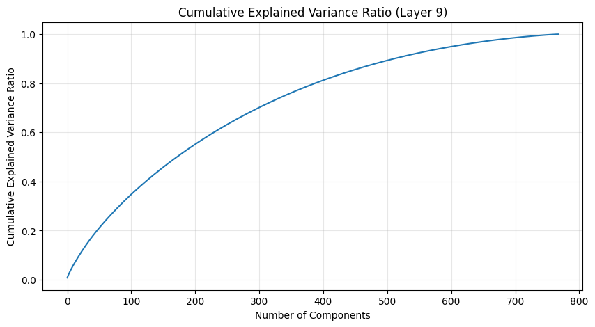
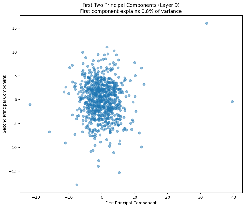
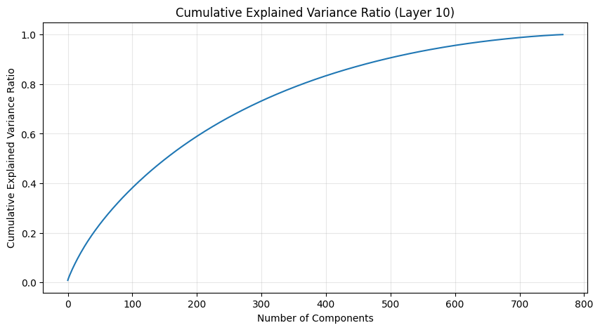
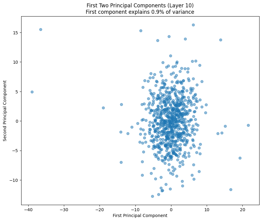
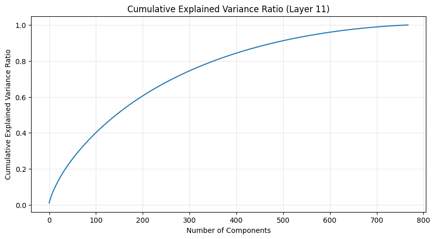
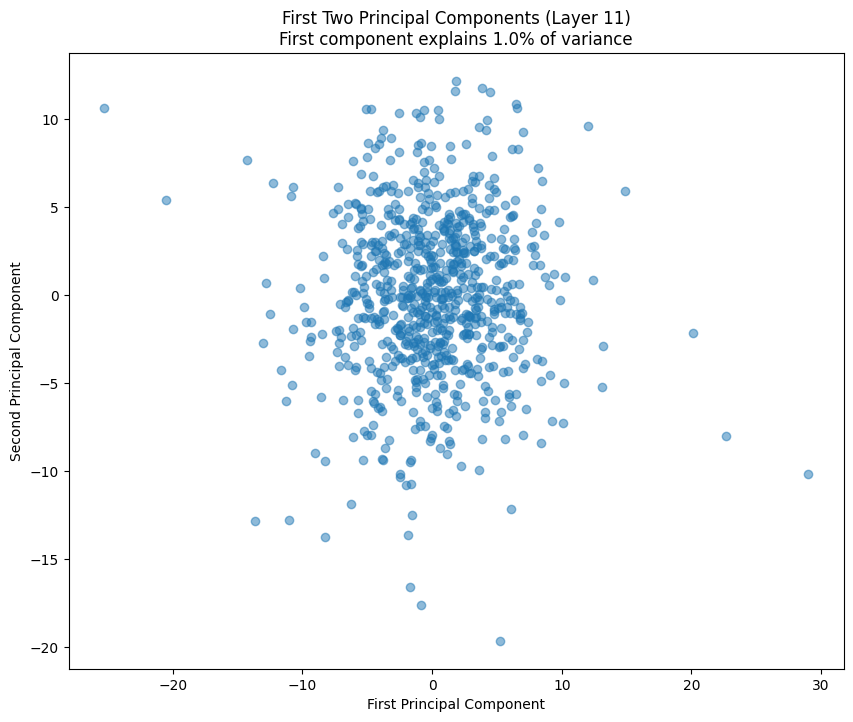
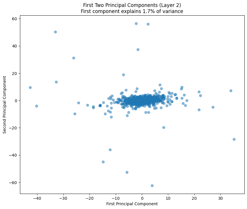
The PCA (Principal Component Analysis) results tell us several important things about the model’s structure:

• The cumulative explained variance shows how many dimensions we really need to capture the weight patterns
• A steep initial curve followed by a long tail suggests the weights operate in a lower-dimensional space than their raw dimensionality
• The scatter plot of the first two components shows how weights cluster in this reduced space
• Clear clusters in this space often indicate specialized weight patterns for different types of features
• The increasing spread in later layers suggests more specialized weight patterns as we go deeper in the network

We can also look at summary stats for the layers.

num_layers = len([k for k in state_dict.keys() if 'h.' in k and 'weight' in k and 'attn.c_attn' in k])
layer_stats = []

for i in range(num_layers):
    weights = state_dict[f'transformer.h.{i}.attn.c_attn.weight'].numpy()
    layer_stats.append({
        'layer': i,
        'mean': np.mean(weights),
        'std': np.std(weights),
        'max': np.max(weights),
        'min': np.min(weights)
    })

# Plot layer-wise statistics
fig, ((ax1, ax2), (ax3, ax4)) = plt.subplots(2, 2, figsize=(15, 10))
fig.suptitle('Layer-wise Weight Statistics', fontsize=16)

layers = range(num_layers)
means = [s['mean'] for s in layer_stats]
stds = [s['std'] for s in layer_stats]
maxs = [s['max'] for s in layer_stats]
mins = [s['min'] for s in layer_stats]

ax1.plot(layers, means, 'o-')
ax1.set_title('Mean Weight Value')
ax1.set_xlabel('Layer')
ax1.grid(True, alpha=0.3)

ax2.plot(layers, stds, 'o-')
ax2.set_title('Weight Standard Deviation')
ax2.set_xlabel('Layer')
ax2.grid(True, alpha=0.3)

ax3.plot(layers, maxs, 'o-')
ax3.set_title('Maximum Weight Value')
ax3.set_xlabel('Layer')
ax3.grid(True, alpha=0.3)

ax4.plot(layers, mins, 'o-')
ax4.set_title('Minimum Weight Value')
ax4.set_xlabel('Layer')
ax4.grid(True, alpha=0.3)

plt.tight_layout()

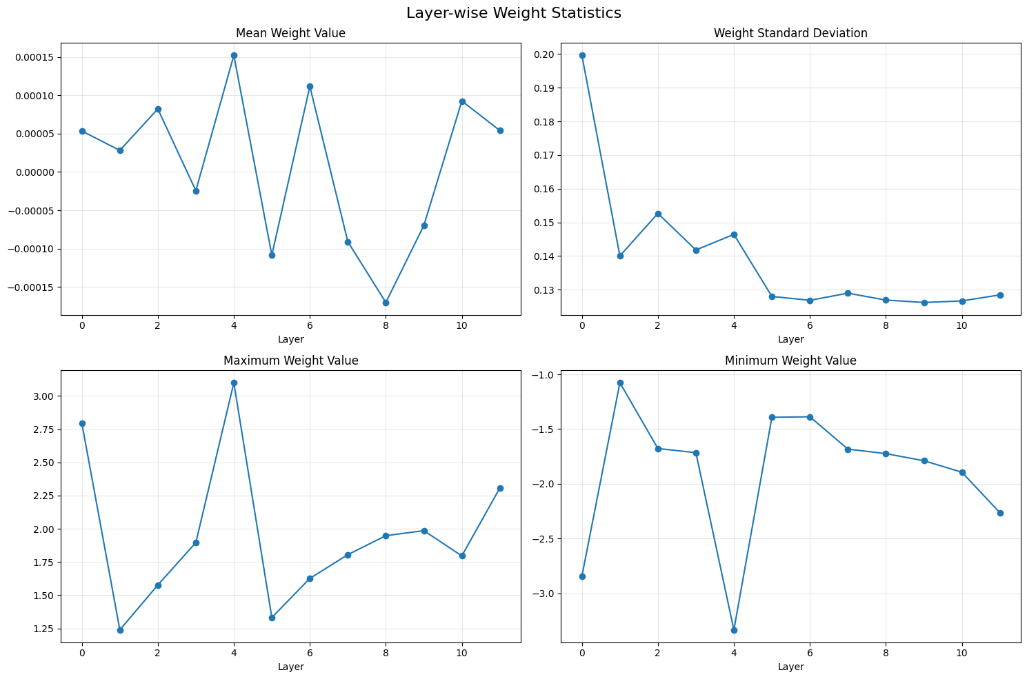
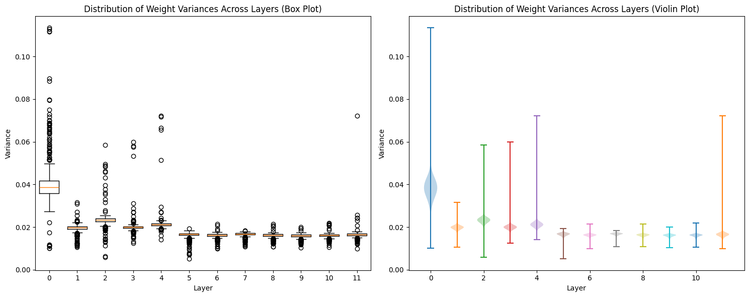
Same with variance:

def get_layer_variance_stats(state_dict):
    layer_variances = []
    for name, param in state_dict.items():
        if 'attn.c_attn.weight' in name:
            layer_idx = int(name.split('.')[2])
            weights = param.numpy()
            variance = np.var(weights, axis=1)
            layer_variances.append((layer_idx, variance))
    return sorted(layer_variances)

layer_variances = get_layer_variance_stats(state_dict)

# Plot distribution of variances across layers
plt.figure(figsize=(15, 6))
for idx, (layer_idx, variance) in enumerate(layer_variances):
    plt.subplot(1, 2, 1)
    plt.boxplot(variance, positions=[layer_idx], widths=0.7)
    
    plt.subplot(1, 2, 2)
    plt.violinplot(variance, positions=[layer_idx])

plt.subplot(1, 2, 1)
plt.title('Distribution of Weight Variances Across Layers (Box Plot)')
plt.xlabel('Layer')
plt.ylabel('Variance')

plt.subplot(1, 2, 2)
plt.title('Distribution of Weight Variances Across Layers (Violin Plot)')
plt.xlabel('Layer')
plt.ylabel('Variance')

plt.tight_layout()

Attention Head Patterns

Finally, let’s look at how attention weights are organized within a single layer:

plt.figure(figsize=(10, 8))
attention_layer = state_dict['transformer.h.0.attn.c_attn.weight'].numpy()
attention_reshaped = attention_layer.reshape(3, -1, attention_layer.shape[1])  # Reshape into Q, K, V
query_weights = attention_reshaped[0]
variance_matrix = query_weights.reshape(12, -1)  # Reshape into attention heads
sns.heatmap(variance_matrix, cmap='viridis')
plt.title('Query Weight Patterns Across Attention Heads (Layer 0)')
plt.xlabel('Weight Index')
plt.ylabel('Attention Head');

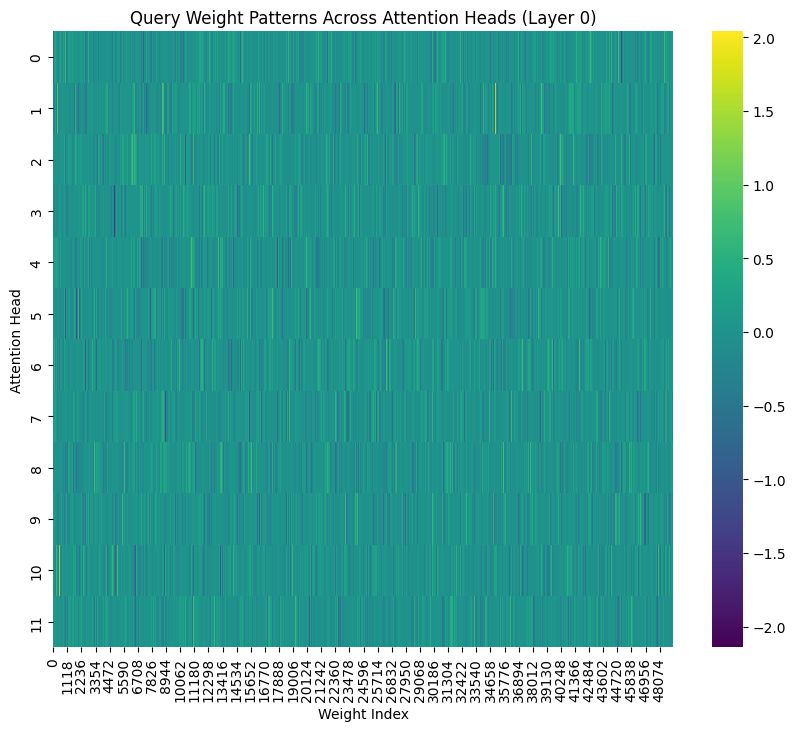
This heatmap shows query weight patterns across different attention heads in the first layer. The vertical axis represents different attention heads, while the horizontal axis shows weight values. Brighter colors indicate higher values. Again, it’s hard to see what’s going on when you look at everything at once.

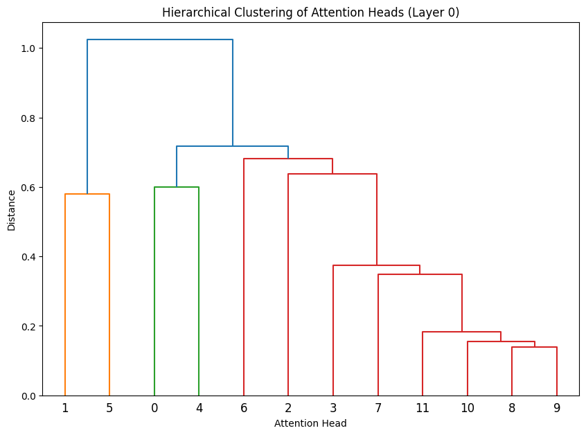
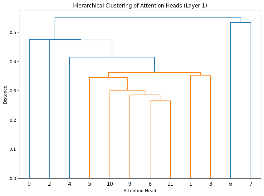
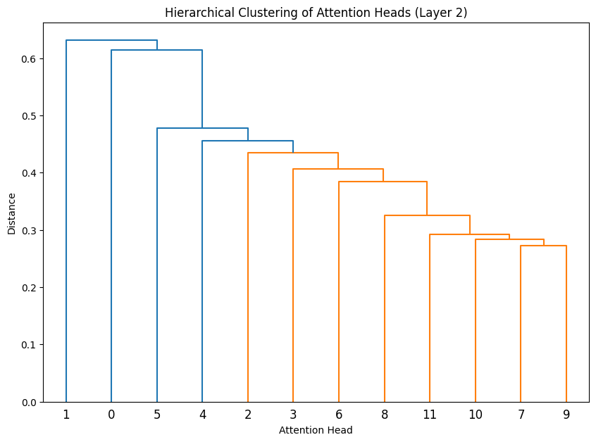
Let’s cluster the attention heads at in different layers.

def cluster_attention_heads(layer_idx):
    weights = state_dict[f'transformer.h.{layer_idx}.attn.c_attn.weight'].numpy()
    head_size = weights.shape[1] // 12
    
    # Get average weight vector for each head
    head_vectors = []
    for i in range(12):
        start_idx = i * head_size
        end_idx = (i + 1) * head_size
        head_weights = weights[:, start_idx:end_idx]
        head_vectors.append(np.mean(head_weights, axis=1))
    
    # Perform hierarchical clustering
    Z = linkage(head_vectors, 'ward')
    
    plt.figure(figsize=(10, 7))
    dendrogram(Z)
    plt.title(f'Hierarchical Clustering of Attention Heads (Layer {layer_idx})')
    plt.xlabel('Attention Head')
    plt.ylabel('Distance')

# Cluster heads in first few layers
for layer_idx in range(3):
    cluster_attention_heads(layer_idx)

# Cluster heads in last few layers
for layer_idx in late_layers:
    cluster_attention_heads(layer_idx)

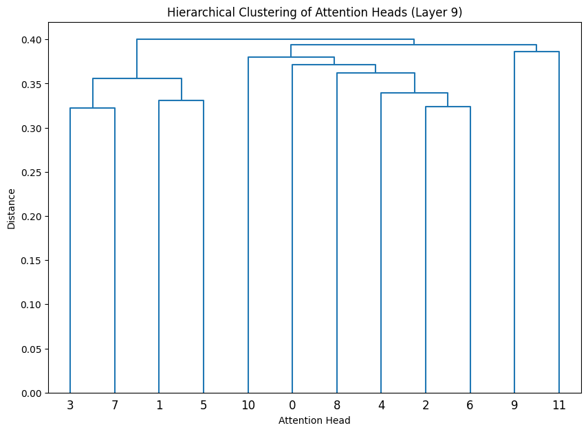
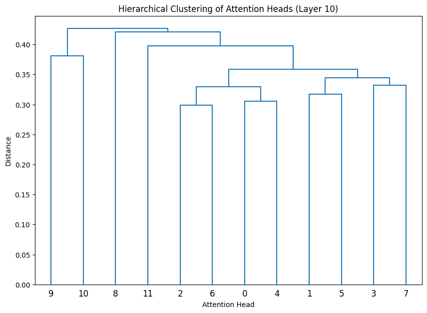
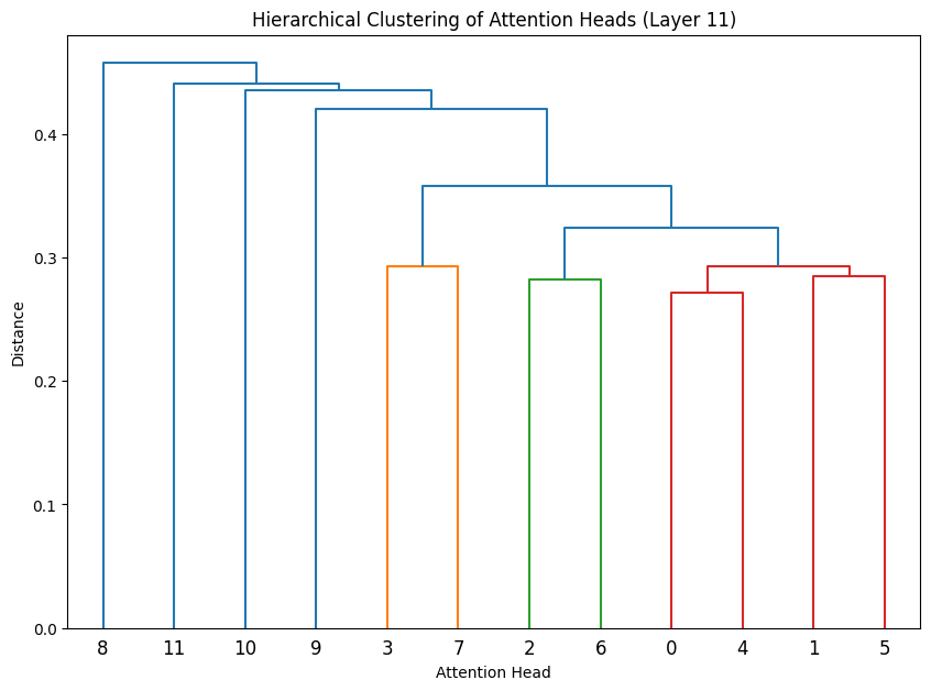
The dendrograms reveal how attention heads cluster based on their weight patterns:

• The height of each connection shows how different the connected heads are
• Heads that cluster together (connected by lower heights) likely have similar functions
• In Layer 0, we see several distinct clusters, suggesting specialized roles early in the network
• The clustering becomes more pronounced in later layers, indicating increasing specialization
• Some heads remain relatively isolated (long vertical lines), suggesting unique specialized functions

Conclusion

There’s lots more to look at, but this gives a basic overview of how you can find structure in these weights. Some of these techniques are pretty useful for determining how well trained a model is.