
In this blog post, I will discuss how to use loss functions in TensorFlow. I’ll focus on binary cross entropy loss.
Table of Contents
import tensorflow.keras.backend as K
import numpy as np
import tensorflow as tf
from matplotlib import pyplot as plt
from tensorflow.errors import InvalidArgumentError

EPSILON = np.finfo(float).eps
Binary Cross Entropy Loss
Let’s imagine the case where we have four different examples that we’ve labeled either 0 or 1, like so:
y_true = np.array([0, 1, 0, 0])
y_pred = np.array([0.1, 0.95, 0.2, 0.6])
Now let’s find the loss.
We’re going to be dealing with logs. Just so we know what we’re using, let’s look at a log plot.
x = np.linspace(0.0001, 1)
y = np.log(x)
plt.plot(x,y);
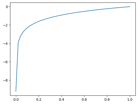
So we’re going to have to take the negative of it. And it also means that for a perfect prediction, we’ll need a value of 1 so there is no loss. So if we’re looking at the 0 class we’ll need to subtract it from 1 to get the correct values.
We’ll get loss from the 0 labels and the 1 labels. Let’s start by doing them separately. We’ll do the ones first.
Here would be the loss from the values if all the labels were 1. You’ll see that the lower predictions have more loss. This makes sense because they are farther away from the true label, which is 1.
np.log(y_pred)
array([-2.30258509, -0.05129329, -1.60943791, -0.51082562])
But we only want the predictions from where the label was 1, so we’ll multiply them by the original predictions.
y_true * np.log(y_pred)
array([-0. , -0.05129329, -0. , -0. ])
Here’s the loss from each individual one. Now let’s combine them.
np.sum(y_true * np.log(y_pred))
-0.05129329438755058
OK. That’s the loss from the ones that should have been a 1. Now let’s find the loss for the ones that should have been 0.
Now, we’re going to take the loss of 1-y_pred.
np.log(y_pred)
array([-2.30258509, -0.05129329, -1.60943791, -0.51082562])
To just get the ones that we didn’t select, we’ll do:
1-y_true
array([1, 0, 1, 1])
Now let’s look at our predictions. The loss will be the distance away from the 0.
np.log(1-y_pred)
array([-0.10536052, -2.99573227, -0.22314355, -0.91629073])
Now we’ll multiply it by 1-y_true to remove the predictions that were correct.
(1-y_true)* np.log(1-y_pred)
array([-0.10536052, -0. , -0.22314355, -0.91629073])
np.sum((1-y_true)* np.log(1-y_pred))
-1.244794798846191
Now that we’ve got the loss from the 0 labels, we’ll combine it with the loss from our 1 labels.
np.sum(y_true * np.log(y_pred)) + np.sum((1-y_true)* np.log(1-y_pred))
-1.2960880932337415
OK, but this number is negative, so it’s not going to work as a loss function that we need to minimize. What we need to do is take the negative of it.
Also, the loss has a 1/N in front of it, so we need to add that.
def bce_loss(y_true, y_pred):
    loss = - 1/(len(y_true)) * (np.sum(y_true * np.log(y_pred)) + np.sum((1-y_true)* np.log(1-y_pred)))
    return loss
print(bce_loss(y_true, y_pred))
0.3240220233084354
Let’s compare this with the loss from TensorFlow.
bce = tf.keras.losses.BinaryCrossentropy(from_logits=False)
bce(y_true, y_pred).numpy()
0.3240218758583069