This post aims to explore decision trees for the NOVA Deep Learning Meetup. It is based on chapter 8 of An Introduction to Statistical Learning with Applications in R by Gareth James, Daniela Witten, Trevor Hastie and Robert Tibshirani. It also discusses methods to improve decision tree performance, such as bagging, random forest, and boosting. There are two posts with the same material, one in R and one in Python.

Table of Contents

• Decision Trees for Regression
  • Overview
  • Data Transformation
  • Building the Decision Tree
  • Regions in Decision Trees
  • Interpreting the Tree
  • Decision Tree Algorithms
    • Building the Tree
  • Pruning
    • Summary
• Decision Trees for Classification
  • Heart Disease Example
• Ensembling for Better Models
  • Bagging
    • Overfitting
    • Out of bag error estimation
    • Summary
  • Random Forests
  • Boosting

Decision Trees for Regression

Decision trees are models for decision making that rely on repeatedly splitting the data based on various parameters. That might sound complicated, but the concept should be familiar to most people. Imagine that you are deciding what to do today. First, you ask yourself if it is a weekday. If it is, you’ll go to work, but if it isn’t, you’ll have to decide what else to do with your free time, so you have to ask another question. Is it raining? If it is, you’ll read a book, but if it isn’t, you’ll go to the park. You’ve already made a decision tree.

Overview

There are good reasons that decision trees are popular in statistical learning. For one thing, they can perform either classification or regression tasks. But perhaps the most important aspect of decision trees is that they are interpretable. They combine the power of machine learning with a result that can be easily visualized. This is both a powerful and somewhat rare capability for something created with a machine learning algorithm.

To see how they work, let’s explore the Hitters database which contains statistics and salary information for professional baseball players. The dataset has a lot of information in it, but we’re just going to focus on three things: Hits, Years, and Salary. In particular, we’re going to see if we can predict the Salary of a player from their Hits and Years.

import pandas as pd
import numpy as np
import matplotlib.pyplot as plt
import pydotplus
from sklearn.externals.six import StringIO  
from sklearn.tree import DecisionTreeRegressor, export_graphviz, DecisionTreeClassifier

Let’s take a quick look at the data.

df = pd.read_csv('data/Hitters.csv', index_col=0)
df.head()

	AtBat	Hits	HmRun	Runs	RBI	Walks	Years	CAtBat	CHits	CHmRun	CRuns	CRBI	CWalks	League	Division	PutOuts	Assists	Errors	Salary	NewLeague
-Andy Allanson	293	66	1	30	29	14	1	293	66	1	30	29	14	A	E	446	33	20	NaN	A
-Alan Ashby	315	81	7	24	38	39	14	3449	835	69	321	414	375	N	W	632	43	10	475.0	N
-Alvin Davis	479	130	18	66	72	76	3	1624	457	63	224	266	263	A	W	880	82	14	480.0	A
-Andre Dawson	496	141	20	65	78	37	11	5628	1575	225	828	838	354	N	E	200	11	3	500.0	N
-Andres Galarraga	321	87	10	39	42	30	2	396	101	12	48	46	33	N	E	805	40	4	91.5	N

First we’ll clean up the data and then make a plot of it. We’re just going to focus on how Years and Hits affect Salary.

df = df.dropna()

fig_size = plt.rcParams["figure.figsize"]
plt.rcParams["figure.figsize"] = (14,10)

font = {'family': 'serif',
        'color':  'k',
        'weight': 'normal',
        'size': 16,
        }

plt.scatter(x=df['Years'], y=df['Hits'], c=df['Salary'], s=40, cmap='inferno')
plt.title("Can Salary be predicted?",
          fontdict=font)
plt.xlabel("Years", fontdict=font)
plt.ylabel("Hits", fontdict=font)
color_bar = plt.colorbar()
color_bar.ax.set_ylabel('Salary (in thousands of dollars)')
plt.show()

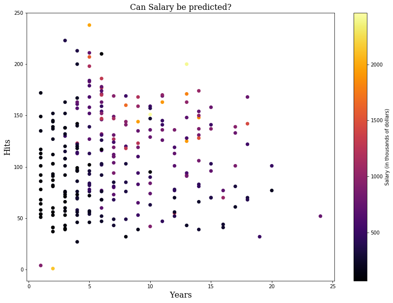
Just from this we can see some outliers with really high salaries. This will cause a right-skewed distribution. One nice thing about decision trees is that we don’t have to do any feature processing on the predictors. We do, however, have to take the target variable distribution into account. We don’t want a few high salaries to have too much weight in the squared error minimization. So to make the distribution more even, we may have to take a log transformation of the salary data. Let’s look at the distribution.

Data Transformation

plt.hist(df['Salary'])

(array([108.,  50.,  49.,  27.,  11.,   7.,   2.,   6.,   1.,   2.]),
 array([  67.5 ,  306.75,  546.  ,  785.25, 1024.5 , 1263.75, 1503.  ,
        1742.25, 1981.5 , 2220.75, 2460.  ]),
 <a list of 10 Patch objects>)

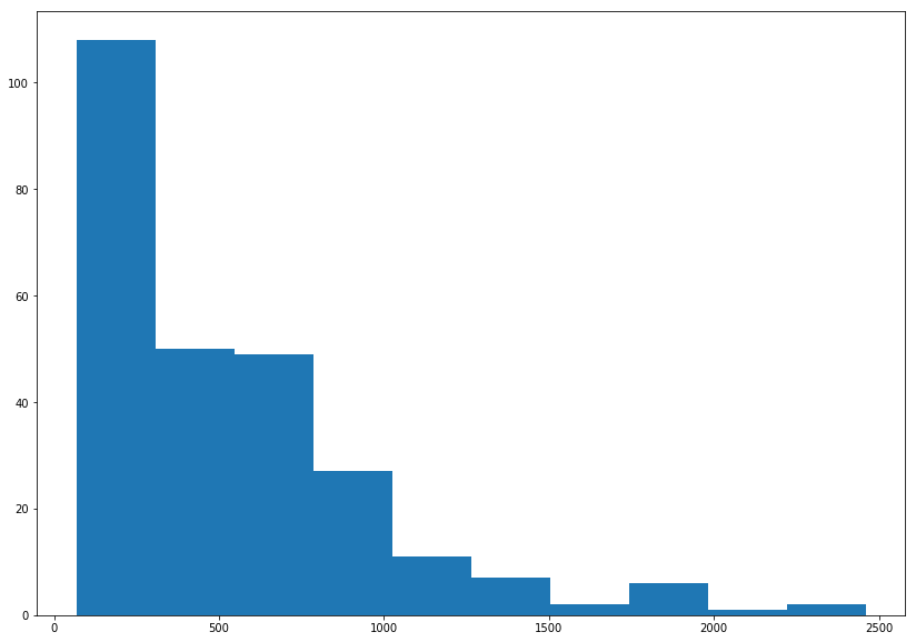
It’s definitely right-skewed. Let’s look at a log transform to see if that’s better.

plt.hist(np.log(df['Salary']))

(array([23., 21., 25., 31., 28., 36., 48., 29., 13.,  9.]),
 array([4.2121276 , 4.5717065 , 4.9312854 , 5.29086431, 5.65044321,
        6.01002211, 6.36960102, 6.72917992, 7.08875882, 7.44833773,
        7.80791663]),
 <a list of 10 Patch objects>)

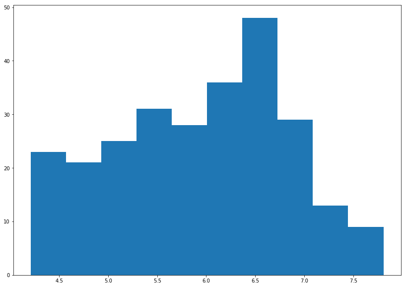
This we can work with. Let’s add this to the dataframe.

Building the Decision Tree

OK, let’s try to predict log.salary based on everything in logHitters (we’ll exclude Salary for obvious reasons).

Here’s the part where the machine learning comes in. Instead of creating our own rules, we’re going to feed all the data into a decision tree algorithm and let the algorithm build the tree for us by finding the optimal decision points.

OK, let’s build the tree. We’ll use the rpart library in R and sklearn in Python.

X = df[['Years', 'Hits']]
y = np.log(df['Salary'])

tree = DecisionTreeRegressor(max_leaf_nodes=3, random_state=0)
tree.fit(X, y)

DecisionTreeRegressor(criterion='mse', max_depth=None, max_features=None,
           max_leaf_nodes=3, min_impurity_decrease=0.0,
           min_impurity_split=None, min_samples_leaf=1,
           min_samples_split=2, min_weight_fraction_leaf=0.0,
           presort=False, random_state=0, splitter='best')

Now let’s take a look at it. In Python we’re going to have to build a helper function to visualize it.

dot_data = export_graphviz(tree,
                           feature_names=['Years', 'Hits'],
                           out_file=None,
                           filled=True,
                           rounded=True,
                           special_characters=True)
graph = pydotplus.graph_from_dot_data(dot_data)
nodes = graph.get_node_list()

graph.write_png('python_decision_tree.png')

True

We’ve made our first decision tree. Let’s go over some terminology. At the top it says Years < 4.5. This is the first decision point in the tree and is called the root node. From there, we see a horizontal line that we could take either to the left or to the right. These are called left-hand and right-hand branches. If we go down the right-hand branch by following the line to the right and then down, we see Hits<117.5 and another decision point. This is called an internal node. At the bottom, we have a few different numbers. Because no more decision points emanate from them, these are called terminal nodes or a leaves. A decision tree will always have one more terminal node than split point. As you can see, the “tree” is actually upside down (perhaps statistician don’t spend enough time outside?).

OK, so now how do we use it?

Let’s go back to the root node where it says Years < 4.5. From here the tree splits into two paths because we’ve reached a decision point. If the statement is true for a given instance, as in the player has fewer than 4.5 Years, we go to the left. There, we see 5.107 and we’ve reached the end of the line. So for players with fewer than 4.5 Years, the model predicts 5.107. Remember that we’re predicting the natural logarithm of the salary in thousands of dollars. So let’s calculate what the actual number would be to see if it makes sense.

print('${:,.0f}'.format(1000*np.exp(5.107)))

$165,174

That looks right. But where did that number come from? When using decision trees for regression, the prediction, 5.107 in this case, comes from taking the mean of all the instances in that category.

Let’s explore what happens for players with more than 4.5 Years. Now we go down the right branch of the and we reach Hits<117.5. Another decision point! Here, if the number of Hits is fewer than 117.5, we go down the left side of the tree to 5.998. If it’s greater than 117.5, we go down the right side to 6.74. Let’s see how much this is.

print('${:,.0f}'.format(1000*np.exp(6.74)))

$845,561

Regions in Decision Trees

Another way to think about decision trees is that they are algorithms that split the input space into different regions. This isn’t particularly easy to see in the tree, so we’ll plot the predictor space.

df.plot('Years', 'Hits', kind='scatter', color='orange', figsize=(7,6))
plt.xlim(0,25)
plt.ylim(bottom=-5)
plt.xticks([1, 4.5, 24])
plt.yticks([1, 117.5, 238])
plt.vlines(4.5, ymin=-5, ymax=250, colors="green")
plt.hlines(117.5, xmin=4.5, xmax=25, colors="green")
plt.annotate('R1', xy=(1.5,117.5), fontsize='xx-large')
plt.annotate('R2', xy=(11.5,60), fontsize='xx-large')
plt.annotate('R3', xy=(11.5,170), fontsize='xx-large');

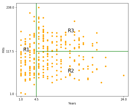
You can see that the predictor space is broken into three regions.

\[R1 ={X | Years< 4.5}\] \[R2 ={X | Years>=4.5, Hits<117.5}\] \[R3 ={X | Years>=4.5, Hits>=117.5}\]

We can see the same tree features here that we saw above. R1, R2, and R3 are the three leaves or terminal nodes. Each decision point results in a line, so you can count the number of lines to get the number of decision points, which are also the number of internal nodes plus the root node.

We make make predictions just as easily with this plot. To make a prediction, we see what region the input falls into, then assign the value to the mean of the entities in that region. So if someone has 10 years and last year had 50 hits, we would put them in R2. The mean logSalary of all our training samples in that region was 5.998, so we’ll predict that value.

Interpreting the Tree

One of the good things about decision trees is that most people already have an intuition about them, so interpretation comes easily. Imagine, for example, that you’re playing 20 Questions. You know the key of the game is to ask good questions up front that help to split the possible solutions into (ideally) two equal sizes. The exact same applies here.

So, why did the tree start with Years? Just like in decision trees for 20 Questions, they start with the most important factor first. This is valuable information; in this case, it tells us that Years is the most important factor in determining logSalary (out of Years and Hits). Then, the next factor is Hits (admittedly these are the only two factors we’re looking at). And Hits has a bigger effect on the Salary of players who have played longer than 4.5 years versus those who haven’t. If we had done a fourth split, it could very well split the less experienced players by Hits as well.

As you might imagine, this model wouldn’t perform particularly well in the real world. On the other hand, it’s got some predictive power and is easy to interpret. That’s an important tradeoff.

Decision Tree Algorithms

Let’s talk a little about how this works mathematically.

Building the Tree

The goal of decision tree algorithms is to find \(J\) regions \(R_1, ..., R_J\) that minimize the RSS given by

\[\sum_{j=1}^{J}{\sum_{i\in R_j}}({y_i-\hat{y}_{R_j}})^2\]

Note that the regions that minimize that equation don’t have to be rectangular, but we’ll impose an addition constraint that they are so that we can can easily interpret the decision points. This means that each question can only be about a single variable. The alternative would be to allow questions like “Is feature 1 times feature 2 greater than 25?” This is not allowed in decision tree implementations. So we’ll assume that each region is a box.

Even so, it would be computational expensive (or even infeasible) to consider every possible partition of the feature space into \(J\) boxes. So instead we use a top-down, greedy approach known as recursive binary splitting. “Top-down” means that it begins at the top of the tree and works its way down. “Greedy” means that it maximizes the value of the split at that particular step, without considering future splits. This is done to make the calculations feasible and may not actually result in the optimal decision tree. It’s possible that a less optimal decision early on allows for much better decisions later, resulting in an overall better tree.

The algorithm continues to create more split points until a stopping condition is met. The stopping conditions are:

1. All the samples have been correctly classified (the leaf nodes are pure)
2. The maximum node depth (set by user) is reached
3. Splitting nodes no longer leads to a sufficient information gain

The three most common algorithms are ID3, C4.5, and CART. They are all similar in some ways but have tradeoffs. ID3 was the first of these to be invented. It had significant limitations, such as it could only handle categorical data, couldn’t handle missing values, and is subject to overfitting. C4.5 is an improved version of ID3. It can handle numeric data as well as missing values and has methods to reduce overfitting. CART (Classification And Regression Trees) is perhaps the most popular decision tree algorithm. It handles outliers better than the other approaches. They all use different criteria to determine a split, which we’ll get into later.

Pruning

So, how big could we make a decision tree? In theory, there is no limit. We could keep building up a decision tree, making it bigger and bigger until every training example is predicted correctly. But this would grossly overfit the data. It turns out that even if we limit the size of the tree by, say, limiting the minimum bucket size, we could still be subject to overfitting. Another way to stop the tree would be to stop when each split decreases the RSS by some threshold. But this has downsides. An unimportant split early on could lead to a better split in the later stages. So what do we do?

The best way to handle overfitting is not to build a small tree, but to build a large tree and prune it. The method used to do this is called “Cost complexity pruning” or “weakest link pruning”. Because there are more powerful methods than pruning a single tree, we’ll just touch on pruning without going into detail on it.

The key to pruning is to add a penalizing factor to the size of the tree (number of terminal nodes in it) just like we do with lasso regression.

For each value of \(\alpha\) there exists a subtree \(T \subset T_0\) where we minimize:

\[\sum_{m=1}^{\vert T\vert}{\sum_{x_i\in R_m}{(y_i-\hat{y}_{R_m})^2+\alpha\vert T\vert}}\]

where

\(\vert T\vert\) - number of terminal nodes in tree \(T\)

\(\alpha\) - the penalty parameter; we can tune this to control the trade-off between the subtree’s complexity and its fit to the training data

\(\sum_{x_i\in R_m}{(y_i-\hat{y}_{R_m})^2}\) - sum of squares in region around region m

\(\sum_{m=1}^{\vert T\vert}\) - add the above sum up for all the terminal nodes

We use cross-validation to find the best alpha, know as \(\hat{\alpha}\). Then we return to the full dataset and obtain the subtree corresponding to the best alpha \((\hat{\alpha})\).

Different decision tree algorithms handle pruning differently. ID3 doesn’t do any pruning. CART uses cost-complexity pruning. C4.5 uses error-based pruning.

Summary

• Use recursive binary splitting to grow a large tree
• Use a stopping criterion, such as stopping when each terminal node has fewer than some minimum number of observations, to stop growing the tree; it’s OK to build a large tree that overfits the data
• Apply pruning to the large tree in order to obtain a sequence of best subtrees, as a function of alpha
• use k-fold cross-validation to find alpha; pick that alpha that minimizes the average error
• Choose the subtree that corresponds to that value of alpha

Let’s go back to the Hitters dataset and see what the optimal tree size is.

X = df.drop(['Salary'], axis=1)
y = np.log(df['Salary'])

league_mapping = {'A': 0, 'N': 1}
division_mapping = {'W': 0, 'E': 1}

def league_let_to_num(col):
    return league_mapping[col]
def divison_let_to_num(col):
    return division_mapping[col]

X['NumericLeague'] = X['League'].apply(league_let_to_num)
X['NumericNewLeague'] = X['NewLeague'].apply(league_let_to_num)
X['NumericDivision'] = X['Division'].apply(divison_let_to_num)

X = X.drop(['League', 'NewLeague', 'Division'], axis=1)

tree = DecisionTreeRegressor(min_samples_leaf = 5, random_state=0)
tree.fit(X, y)

DecisionTreeRegressor(criterion='mse', max_depth=None, max_features=None,
           max_leaf_nodes=None, min_impurity_decrease=0.0,
           min_impurity_split=None, min_samples_leaf=5,
           min_samples_split=2, min_weight_fraction_leaf=0.0,
           presort=False, random_state=0, splitter='best')

dot_data = export_graphviz(tree,
                           out_file=None,
                           filled=True,
                           rounded=True,
                           special_characters=True)
graph = pydotplus.graph_from_dot_data(dot_data)
nodes = graph.get_node_list()

graph.write_png('python_full_decision_tree.png')

True

Image from ISLR.

Looks like a tree size of three is best. “Tree Size” in this case is the number of terminal nodes.

Decision Trees for Classification

Now let’s talk a little bit about using decision tree for classification, which are sometimes called classification trees. Most of the concepts mentioned above apply equally well to classification trees, so let’s focus on the differences.

The first difference is that we’ll be classifying inputs into a category instead of predicting a value for them. This works as you might expect. Instead of taking the mean of all the instances in a region, we’ll have those instances all vote, and use majority wins to determine what to classify new samples in that region.

Because we’re doing classification, we can’t use the same loss function as before. The most obvious substitute would be to find the fraction of training observations in a particular region don’t belong to the majority class, then subtract that to get the error. This is called the classification error rate.

This can be written mathematically as:

\[E=1-max_k(\hat{p}_{mk})\]

Here \(\hat{p}_{mk}\) represents the proportion of training observations in the \(m\)th region that are from the \(k\)th class.

Although this may be the most straightforward method of identifying error, it isn’t always the most effective. Two other measures of impurity are common used: The Gini index and cross-entropy. Here are the formulas for them:

Gini index:

\[G=\sum_{k=1}^{K}{\hat{p}_{mk}}(1-\hat{p}_{mk})\]

Cross-enropy:

\[D=-\sum_{k=1}^{K}{\hat{p}_{mk}}\log\hat{p}_{mk}\frac{1}{2\log(2)}\]

Note that we’ve added a scaling factor to the cross-entropy function to make it easier to compare with the other methods.

The Gini index (also called Gini coefficient) and cross-entropy are common used measures of impurity. Gini index is the default criterion for scikit-learn.

Let’s look at an example. Say there are ten instances in a region, three of which are labeled as True and seven of which as labeled as False.

To calculate the classification error rate, we can see that the majority class, \(k\), is False. Thus, \(\hat{p}_{mk}\), the proportion of observations in this region that are False, is 0.7. So the final classification error rate would be \(E = 1 - 0.7 = 0.3\).

The Gini index in the above scenario would be \(0.7*0.3 + 0.3 * 0.7 = 0.21 + 0.21 = 0.42\).

The cross-entropy is harder to calculate by hand so we’ll plug it into the computer.

-((0.7 * np.log(0.7)) + (0.3 * np.log(0.3)))/ (2*np.log(2))

0.44064544961534635

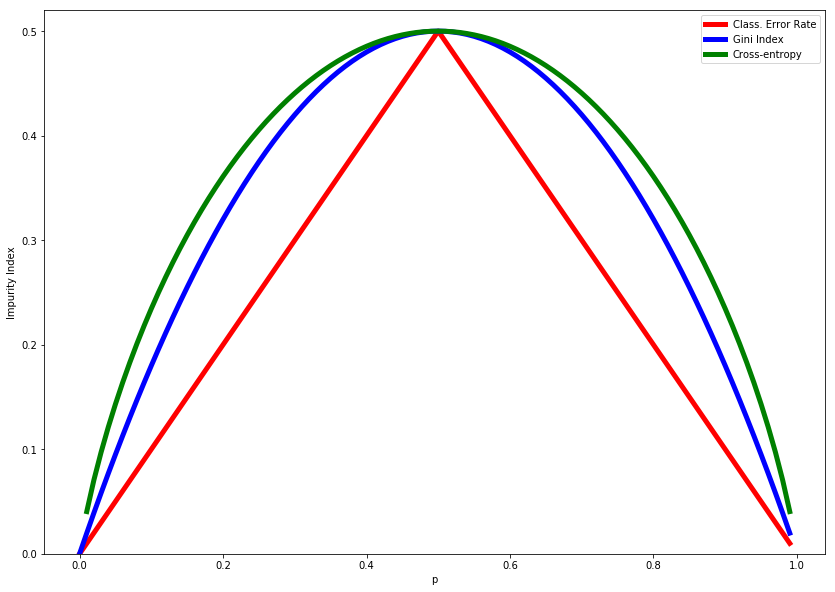
Note that the (scaled) cross-entropy is the greatest, then the Gini index, then the classification error rate. If we plot the formulas, we’ll see that this is what we should expect.

def classification_error(p):
    return 1 - np.max([p, 1 - p])

def gini(p):
    return 2*(p)*(1 - p)

def entropy(p):
    return (p*np.log((1-p)/p) - np.log(1 - p)) / (2*np.log(2))

x = np.arange(0.0, 1.0, 0.01)
class_error_vals = [classification_error(i) for i in x]
gini_vals = gini(x)
entropy_vals = [entropy(i) if i != 0 else None for i in x]

fig = plt.figure()
ax = plt.subplot()

for j, lab, c, in zip(
    [class_error_vals, gini_vals, entropy_vals],
    ['Class. Error Rate', 'Gini Index', 'Cross-entropy'],
    ['red', 'blue', 'green']):
    line = ax.plot(x, j, label=lab, linestyle='-', lw=5, color=c)

ax.legend(loc='upper right', fancybox=True, shadow=False)

plt.ylim([0, 0.52])
plt.xlabel('p')
plt.ylabel('Impurity Index')
plt.show()

Heart Disease Example

Let’s look at an example using heart disease data.

df2 = pd.read_csv('data/Heart.csv', index_col=0)
df2 = df2.dropna()

df2.ChestPain = pd.factorize(df2.ChestPain)[0]
df2.Thal = pd.factorize(df2.Thal)[0]

X2 = df2.drop('AHD', axis=1)
y2 = pd.factorize(df2.AHD)[0]

tree = DecisionTreeClassifier(max_depth=None, max_leaf_nodes=6, max_features=3, random_state=0)
tree.fit(X2,y2)

DecisionTreeClassifier(class_weight=None, criterion='gini', max_depth=None,
            max_features=3, max_leaf_nodes=6, min_impurity_decrease=0.0,
            min_impurity_split=None, min_samples_leaf=1,
            min_samples_split=2, min_weight_fraction_leaf=0.0,
            presort=False, random_state=0, splitter='best')

dot_data = export_graphviz(tree,
                           feature_names=X2.columns,
                           out_file=None,
                           filled=True,
                           rounded=True,
                           special_characters=True)
graph = pydotplus.graph_from_dot_data(dot_data)
nodes = graph.get_node_list()

graph.write_png('python_heart_disease_decision_tree.png')

True

Ensembling for Better Models

Decision trees are often not as successful as some of the other methods. So we’ll also talk about bagging, random forests, and boosting. Each of these is a method to produce and combine multiple trees to that gives a single prediction.

Although decision trees can be powerful machine learning models, they often don’t match up against other models, such as support vector machines. But there’s a way to make up for this by combining the output of several algorithms into a single classifier. This is known as ensembling.

Any machine learning model can be combined with others in an ensemble, so these techniques are not specific to decision trees. However, decision trees have many properties that make them especially good for ensemble learning.

The most popular techniques for ensemble learning are bagging, random forest, and boosting. They can all be used with decision trees to build more powerful models.

Bagging

Heavily trained decision trees can often suffer from high variance. This means that if we build a decision tree of off two halves of the same dataset, they could have significant differences. This might sound like a negative, and it is, but we can also use it to our benefit. The high variance between the models allows us to combine decision trees to make better predictions. If the variance were low, we wouldn’t gain much from combining models trained from different data sets. Overall, this can significantly improve the accuracy of your model. Let’s talk about a few ways we can do that.

The first is called bagging, which comes from bootstrap aggregation. Its job is to reduce the variance of a model.

Bagging relies on an important concept in statistics. Recall that if you have \(N\) observations, each of which has a variance of \(\sigma^2\), then the variance of the mean will be \(\sigma^2/N\). We’ll we can use the same principle here. In bagging, we take our single training set and generate B different bootstrapped sets by taking a random sample with replacement. Then we make B decision trees each making their own prediction. Then we average those predictions into a final answer.

Mathematically, it looks like this:

\[\hat{f}_{avg}(x)=\frac{1}{B}\sum_{b=1}^B{\hat{f}^b(x)}\]

When bagging with regression, you take the average of all the resulting predictions. For classification, simply take a majority vote.

Overfitting

One of the great aspects of bagging is that creating more trees does not result in overfitting. Not only that, but you can input large, overfit trees that haven’t been pruned. The variance in the different trees will balance each other out. You can use hundreds or even thousands of trees to average. The way to determine the number of trees is to watch when your accuracy stops decreasing.

Out of bag error estimation

How do we estimate the error? There’s actually an easy way to do this and you don’t need to use cross validation. It’s called out-of-bag error estimation. Imagine the following situation.

If there are N training examples in total and you choose N examples for each bagged dataset, you will almost certainly have duplicates of some (because you’re replacing them each time) and have completely missed others. In fact, on average you will have \(1-\frac{1}{e} \approx 0.632\) of the example in the original dataset appear in the bagged one. That leaves another 36.8% of the data in the original training set that your model has never seen. These are called out-of-bag (OOB) instances because they aren’t included in the bagged set. And because your model hasn’t seen them, then they can be used as a test set to get an accuracy score.

We’ll take the OOB values and generate predictions with them. Then we’ll use the predictions to calculate the error (mean squared error for regression and classification error for classification). This gives us a good way to measure the error.

Summary

Bagging is a great option for combining models with high variance, and decision trees are a great use-case. Even more, bagging doesn’t lead to overfitting. However, there’s a significant downside as well. One of the greatest benefits of decision trees is their interpretability. That interpretability is lost when bagging is used. There’s no longer any way to display the model or easily show how a decision was made.

However, you can still find the most important predictors, either in terms of RSS for regression trees or Gini index for classification trees.

Random Forests

Another powerful technique is known as random forests. Random forests offers an improvement over bagged trees because it allows us to decorrelate the trees. We start the same way as in bagging - build a number of decision trees based on bootstrapped training samples. But each time there’s a split, we only allow a random subset, \(m\), of the \(p\) predictors to be chosen as split candidates. So if we’re looking at the baseball dataset again, for a particular split you might only to able to split based on Hits and Runs, but not Home Runs or RBIs. For a dataset with \(p\) different features, \(m\) is typically chosen such as \(m \approx \sqrt{p}\).

So this means we work with less than half of the features. This means we often don’t use the strongest predictor as our first split. \((p - m) / p\) of the time the strongest predictor won’t even be available. This makes the trees more varied.

Note that bagging is actually just a subset of random forests. Specifically, it is a random forest with \(m=p\).

The more correlated the different features are the lower the value of m we should use.

Again, more trees won’t cause more overfitting. The key to determining the number of trees is to see when the error rate settles down.

Boosting

Now let’s talk about a technique known as boosting. Boosting is another way we can improve decision tree performance. Like the other techniques, it can be applied to many machine learning models, but is most commonly used with decision trees. We’re going to focus on boosting regression trees but the concept is the same for classification trees.

This process does not involve bootstrapping - we’ll train the decision trees on the entire dataset. But then we’ll take the output from that and input it into a second tree. Thus the output of one model will be fed into the next. We fit a decision tree to the residuals from the previous model. Then use update the residuals and do it again.

These trees can be quite small, maybe with just a few nodes in them. By adding these small trees, we gradually improve the overall model in the areas where it needs the most help.

There are three parameters of primary interest when boosting:

\(B\) - the number of trees. Unlike in bagging and random forests, boosted model can overfit. This means you will need to limit \(B\). Use cross-validation to find the optimal number for \(B\).

\(\lambda\) - the shrinkage parameter. This is like the learning rate in other algorithms. It determines the rate at which the model learns.

\(d\) - the number of splits in the tree. This controls the complexity of each tree. Often, numbers as low a 1 work well for boosting.

The final boosted model looks like:

\[\hat{f}(x)=\sum_{b=1}^B{\lambda\hat{f}^b(x)}\]

I like to think of boosting as working in series, while bagging works in parallel.