
Now that we’ve cleaned and prepared the data, let’s try classifying it using logistic regression. Logistic regression is a popular machine learning algorithm for classification due to its speed and accuracy relative to its simplicity.
Logistic regression is like linear regression in that it tries to find an appropriate way to weigh every input. After multiplying each input by its respective weight, a bias is applied. Then the result is put into a nonlinear activation function and a prediction is made based on the result.
How on Earth could that work? Well, what I’ve described so far would never work, but here is where the machine learning comes in. For our first iteration, we’ll only get about half right (in the case of two possible outputs). But we back propagate the difference between the correct answers and our results through the algorithm to update our weights. Then we’ll make another set of predictions. Then we do it again. And again. Eventually, the weights will become tuned well enough to accurately make predictions. Let’s see how it works.
Table of Contents
import pandas as pd
import numpy as np
import matplotlib.pyplot as plt
from sklearn.model_selection import train_test_split
X = np.load('dna_cleaner.npy')
y = np.load('dna_clean_labels.npy')
print(X.shape)
print(y.shape)
(3190, 287)
(3190,)
We could do one vs. many, but we’re not going to. We’re going to skip the instances that don’t contain either introns or extrons. This will simplify things. Let’s see where they are and how they’re distributed in the dataset.
np.where(y==2)
(array([1535, 1536, 1537, ..., 3187, 3188, 3189], dtype=int64),)
Fortunately, they’re in order at the end, so this makes removing them much faster. We just truncate the array.
X = X[:1535]
y = y[:1535]
print(X.shape)
print(y.shape)
(1535, 287)
(1535,)
Preparing the Data
We randomly split the data into training and testing sets.
X_train, X_test, y_train, y_test = train_test_split(X, y, test_size=0.25, random_state=0)
X_train.shape
(1151, 287)
num_inputs = X.shape[0]
input_size = X.shape[1]
A Single Example
Initializing Parameters
After we have the data the next step is to initialize the parameters we’ll need. We will need a weight parameter for each input and a bias parameter. The easiest way to do this is to initialize them all to zero using np.zeros(). They will become nonzero after the first iteration.
def initialize_parameters(input_size):
    # Weights can all start at zero for logistic regression
    weights = np.zeros(input_size,)
    # For any kind of network, we can initialize the bias to zero
    bias = np.zeros(1)
    return (weights, bias)
weights, bias = initialize_parameters(input_size)
We have to be very careful with our matrix sizes. Let’s look at the shape of the ndarrays.
print("The weight parameter is of shape: " + str(weights.shape))
print("The bias parameter is of shape: " + str(bias.shape))
The weight parameter is of shape: (287,)
The bias parameter is of shape: (1,)
So weights and bias are both 1-dimensional arrays (n,). When we add anything to them we’ll have to make sure the shape matches.
Forward Propagation
Now that we’ve initialized our variables, it’s time to make an initial calculation. We’re going to take each input value and multiply it by a weight. Then we’ll sum the weights together and add a bias. The bias term can make one outcome more likely than another, which helps when there is more of one outcome than another (such as cancer vs. not cancer in diagnostic imagery).
Here is how it works mathematically:
\[Z = w_0x_0 + w_1x_1 + ... w_mx_m\]where
-
\(Z\) is the sum of the weighted inputs
-
\(w_0\) is the initial weight, often known as the bias
-
\(x_0\) is 1 to allow for the bias \(w_0\)
-
\(w_1\) is the weight associated with the first input
-
\(x_1\) is the first input
-
\(w_m\) is the weight associated with the last input
-
\(x_m\) is the last input
Thus we can map any value of x to a value for y between 0 and 1. We can then ask if the result is greater than 0.5. If it is, put it in category 1, if not, category 0. And we’ve got our prediction. The tricky part, however, is to find the correct weights.
Let’s make sure there is a weight for every element in the image. The shapes of the ndarrays must be the same.
assert X_train[0].shape == weights.T.shape
Alright, let’s do the actual calculations. Even though the bias is zero for the first iteration we’ll include it here for completeness.
image_sum = np.dot(weights, X_train[0]) + bias
image_sum
array([0.])
The result is going to be zero because we initialized all the weights to zero. It won’t be zero once we update our weights.
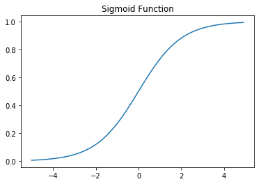
After \(Z\), the sum of the weighted input (image_sum in the code), has been determined, we need to convert that value into a class. The trick is to use an activation function. The term “activation function” comes from neurons with the brain, which will activate if they have sufficient electrical stimulation (roughly speaking). For our purposes, the activation function is going to translate \(Z\), which can be \(-\infty\) to \(\infty\), into a value between 0 and 1.
To do this, we will use a sigmoid function.
\[S(z) = \frac{1}{1+e^{-z}}\]where
-
\(S(z)\) is an output between 0 and 1
-
\(z\) is the input (or the sum of the model inputs in the case of logistic regression)
They create an S-shaped curve.
def sigmoid(z):
    s = 1/(1+np.exp(-z))
    return s
x_sigmoid = np.arange(-5, 5, .1)
y_sigmoid = sigmoid(x_sigmoid)
plt.plot(x_sigmoid,y_sigmoid)
plt.title('Sigmoid Function')
plt.show()
In some notations, the output is written as A or y-hat. In our case, we’ll just call it output.
output = sigmoid(image_sum)
print(output)
[0.5]
To predict the actual label, we’ll set the cutoff to 0.5, so we map all values above 0.5 to 1.0 and all below 0.5 to 0.
Side note: Numpy uses the IEEE 754 standard for rounding, which states that values halfway between two numbers (e.g. 0.5, 1.5) should be rounded towards the even number. Thus 0.5 will be rounded to 0. Here’s a quick demo:
for i in [0.5, 1.5, 2.5, 3.5]:
    print(np.round(i))
0.0
2.0
2.0
4.0
Back to logistic regression. Now we make the predictions.
y_prediction = np.rint(output).astype(int)  # this forces either 0 or 1
print(y_prediction)
[0]
Let’s compare our prediction with the true value.
y_train[0]
1
It doesn’t particularly matter whether our prediction was accurate or not. We’re actually comparing the output against the correct answer and not the y_prediction. We do this because if the output was, say, 0.51, it would round to 1. This may be correct, but the fact that the model thought that was only a 0.51 and not 1.0 or at least > 0.90 shows that it still needs to be trained.
Now we’ll use the error to update our weights in a process known as back propagation.
Back Propagation
In this part, we have to calculate the partial derivatives \(\frac{\partial \mathcal{L}}{\partial w}\) and \(\frac{\partial \mathcal{L}}{\partial b}\).
To refine the weights, we have to find what guesses were wrong and impose a cost for those errors. There are lots of functions, known as either loss functions or cost functions, that could do this. For example, we could use squared error (also known as L2 loss), which looks like this:
\[\mathcal{L}(a,y) = (a-y)^2\]But because the prediction function is nonlinear (due to the activation function), this loss function will give us many local minima. To ensure that gradient descent can find the absolute minimum, we must avoid this. In turns out that the best loss function to use to help gradient descent is the log-likelihood function:
\[\mathcal{L}(a,y) = -(y \log a+(1-y)\log(1-a))\]where
-
\(L\) is the loss from a single example. There are many notations for loss functions.
JandCare also commonly used to represent the loss function. -
\(y\) is the class true label. It is either a zero or a one.
-
\(a\) is the output from the activation function.
This loss function looks more complex than it is. Because the value of y is either a 0 or 1, one of the two terms will disappear. This function is equivalent to saying:
If y = 0:
\(\mathcal{L}(a,y) = -(\log(1-a))\)
If y = 1:
\(\mathcal{L}(a,y) = -(\log a)\)
OK, let’s see what our loss is.
loss = -(y_train[0] * np.log(output) + (1-y_train[0])*np.log(1-output))
loss
array([0.69314718])
But the total amount of loss isn’t particularly useful unless we know how much of it to attribute to the bias and to the respective weights. To find that, we’ll look at how the cost function varies with changes in the weight and the bias. That is, we’ll have to calculate the partial derivative of the cost function with respect to these variables.
\[\frac{\partial \mathcal{L}}{\partial w} = x(a-y)\]where
-
\(\frac{\partial \mathcal{L}}{\partial w}\) is the change in the cost function due to the change in the weight parameters
-
\(x\) is the input
-
\(a\) is the output of the activation function
-
\(y\) is the true value
Something interesting to note: By multiplying by the input size as well, we change the weights more for inputs that had high values, so the algorithm automatically finds the most significant weights and changes them.
Similarly, for the bias we have:
\[\frac{\partial \mathcal{L}}{\partial b} = (a-y)\]The Fast.ai wiki has a good guide on log loss functions. There are also far more detailed explanations and derivations of these in chapters 2 and 3 of Neural Networks and Deep Learning, as well as in Andrew Ng’s Coursera course on Neural Networks and Deep Learning.
We don’t want our weights to swing widely each time we get a new value, so we’ll introduce a small learning rate that we can use to reduce the step size. If the step size is too large, we won’t be able to find the minimum.
learning_rate = 0.001
weights[0] = weights[0] + learning_rate * loss * X_train[0][0]
Now we continue to do that for every weight in our algorithm.
weights[1] = weights[1] + learning_rate * loss * X_train[0][1]
Obviously, doing this one by one isn’t a good idea, so we’ll write a loop that goes through all the samples.
So let’s reset the weights then do them all at the same time.
All examples
In the example above, we took a single instance and propagated it forward and backward through the network. If we were going to continue to do that it would be important to randomize the order that the instances propagate through the model. But that’s not actually how we’re going to run data through the model. Instead, we’ll simultaneously propagate all instances forward through the model at the same time, then simultaneously backward through the model. This is called “batch learning”.
We’ll start over again with a new set of weights and a bias.
Initialize
weights, bias = initialize_parameters(input_size)
Now use the vectorization in numpy to calculate the output for every single instance.
Forward Propagation
outputs = sigmoid(np.dot(weights,X_train.T) + bias)
outputs.shape
(1151,)
Now let’s make our predictions.
y_prediction = np.rint(outputs).astype(int) # this forces either 0 or 1
y_prediction[:10]
array([0, 0, 0, 0, 0, 0, 0, 0, 0, 0])
Because all of our weights were the same, all the results will be the same. This will change after we’ve backwards propagated through the algorithm once.
Backpropagation
To find the total cost, we have to sum through all cases and then divide by the number of cases.
\[J(a,y) = -\frac{1}{n}\sum_{i=1}^{n}y^{(i)}\log(a^{(i)})+(1-y^{(i)})\log(1-a^{(i)})\]where
-
\(J(a,y)\) is the total loss. \(J = \sum \mathcal{L}\)
-
\(n\) is the number of inputs, that is, the number of different DNA sequences
\(a^{(i)}\) is the output of the activation function of the \(i^{th}\) DNA sequence
\(y^{(i)}\) is the true value of the \(i^{th}\) DNA sequence
Vectorization
However, instead of summing through each instance, we’re going to calculate these as vectors:
\[J(A,Y) = -(Y \log A+(1-Y)\log(1-A))\]where
-
\(J(A,Y)\) is the total loss
-
\(Y\) is a vector of all true class labels.
-
\(A\) is a vector of the output of all activation functions
We’ll record the total cost because we should see it decrease over training epochs. But again it’s actually not the number that we’ll mostly be dealing with. It’s the partial derivatives that we’re interested in. We’ll calculate them again.
\[\frac{\partial J}{\partial w} = \frac{1}{n}X^T(A-Y)^T\]where
-
\(\frac{\partial J}{\partial w}\) is the change in the total cost as the weight changes
-
\(n\) is the number of inputs
-
\(X\) is a vector of all inputs
-
\(A\) is a vector of all the outputs of the activation function
-
\(Y\) is a vector of all true class labels
Note that depending on the shape of the matrices, it may be necessary to transform some of them before you can take their dot product.
And we do the same for the bias
\[\frac{\partial J}{\partial b} = \frac{1}{n} \sum (A-Y)\]OK, let’s do the code.
cost = (-1/num_inputs) * np.sum(y_train*np.log(outputs) + (1-y_train)*np.log(1-outputs))
To simply the code, we’ll call dJ/dw just dw and dJ/db just db.
dw = (1/num_inputs) * np.dot(X_train.T, (outputs-y_train).T)
dw.shape
(287,)
dw[:10]
array([ 0.0019544 , -0.00944625,  0.01498371, -0.01433225,  0.        ,
        0.00065147, -0.0009772 ,  0.00423453, -0.01074919,  0.        ])
As you can see, even though the weights all started the same, because of the variation in the input the resulting changes to the weights differ. This means once we update the weights they will be different.
OK, now we have a cost associated with every weight. Let’s do the same for the bias.
db = (1/num_inputs) * np.sum(outputs-y_train)
db
-0.0068403908794788275
OK, now we have our gradients. Let’s update the weight and bias.
assert weights.shape == dw.shape
weights = weights - learning_rate * dw
bias = bias - learning_rate * db
Building a Model
Cool. Now we’ve been through an entire forward and backward propagation of a logistic regression model. The weights are still very untrained, so we’ll have to go through many epochs to refine them. Let’s build a function to do that.
def model(X_train, y_train, epochs=500, learning_rate=0.1):

    num_inputs = len(X_train)

    # Create an empty array to store predictions
    y_prediction = np.empty(num_inputs)

    weights, bias = initialize_parameters(input_size)

    for i in range(epochs):

        # Now we calculate the output
        # We're doing this for all images at the same time
        image_sums = np.dot(weights, X_train.T) + bias
        # Now we have to run each output through our activation function, then convert it to a prediction
        outputs = sigmoid(image_sums)
        # Now we have to convert the outputs to predictions
        # round it to an int
        y_prediction = np.rint(outputs).astype(int)  # this forces either 0 or 1

        # Find weight and bias changes
        dw = (1/num_inputs) * np.dot(X_train.T, (outputs-y_train).T)
        dw = np.squeeze(dw)
        db = (1/num_inputs) * np.sum(outputs-y_train)
        # Update the parameters
        # Make sure the matrices are the same size
        assert weights.shape == dw.shape
        weights = weights - learning_rate * dw
        bias = bias - learning_rate * db

    parameters = {"weights": weights,
                  "bias": bias,
                  "train_predictions": y_prediction,
                  }

    return parameters
results = model(X_train, y_train, epochs=300)
Now that we’ve trained all the weights, let’s make predictions against the test set.
final_weights = results['weights']
final_bias = results['bias']
final_sums = np.dot(final_weights, X_test.T) + final_bias
final_outputs = sigmoid(final_sums)
test_predictions = np.rint(final_outputs).astype(int)  # this forces either 0 or 1
train_predictions = results['train_predictions']
print("Accuracy on training set: {:.2%}".format(1-np.mean(np.abs(train_predictions - y_train))))
print("Accuracy on testing set: {:.2%}".format(1-np.mean(np.abs(test_predictions - y_test))))
Accuracy on training set: 98.26%
Accuracy on testing set: 96.88%
And that’s how logistic regression works!