Convolutional neural networks (CNNs) are the powerhouse behind modern computer vision. And although they’ve grown in popularity with the rise of deep learning, they long predate it. In fact, CNNs have long been used with hand-crafted filters. These filters are used to extract specific components of an image which can then be used to understand what is in the image. This post demonstrates some of the most popular filters used in traditional computer vision. You’ll notice that in deep learning the word “filter” is sometimes used interchangeably with the word “kernel”. We’ll use both terms here as well.
Table of Contents
Convolutional Operations
To demonstrate how these convolutional operations work we’ll write out the code for it. These implementations are made to be illustrative and are not the most efficient solutions. For more efficient solutions, we’ll demonstrate the scipy libraries.
We’ll start with a simple convolutional operation between an identically sized kernel and receptive field. First, what do we mean by a convolutional operation? Technically, the “convolutional” operation used in convolution neural networks isn’t actually a convolution but is instead a cross-correlation. Let’s look at an example. Say we have the following matrices:
\[M_x = \begin{bmatrix} x_1 & x_2 & x_3\\ x_4 & x_5 & x_6\\ x_7 & x_8 & x_9 \end{bmatrix}\] \[M_y = \begin{bmatrix} y_1 & y_2 & y_3\\ y_4 & y_5 & y_6\\ y_7 & y_8 & y_9 \end{bmatrix}\]The convolutional operation as used in deep learning is the following:
\[M_x \ast M_y = x_1y_1 + x_2y_2 + x_3y_3 + x_4y_4 + x_5y_5 + x_6y_6 + x_7y_7 + x_8y_8 + x_9y_9\]In mathematics these are called cross-correlations, but in the field of machine learning, this is a convolutional operation.
For completeness, here is what a mathematical correlation would be:
\[M_x \star M_y = x_1y_9 + x_2y_8 + x_3y_7 + x_4y_6 + x_5y_5 + x_6y_4 + x_7y_3 + x_8y_2 + x_9y_1\]OK. Let’s code it up.
Code
Here is the code for a deep learning convolution.
import numpy as np
from matplotlib import pyplot as plt
from PIL import Image
from scipy.signal import correlate2d, convolve2d
def conv(receptive_field: np.ndarray, kernel: np.ndarray, mathematical_convolution: bool = False) -> float:
    """
    Convolve a kernel with an identically-sized receptive field. Option to perform mathematical convolution instead.

    Arguments:
        receptive_field -- Section of array to be convolved
        kernel -- Convolutional filter (aka kernel)

    Keyword Arguments:
        mathematical_convolution -- Assign to true to perform a mathematical convolution (default: {False})

    Returns:
        Scalar return of convolutional operation
    """
    receptive_field_shape = receptive_field.shape
    kernel_shape = kernel.shape
    assert len(kernel_shape) == 2, f"Only two dimensional kernel is allowed, not {len(kernel_shape)}"
    assert len(receptive_field_shape) == 2, f"Only two dimensional matrix is allowed, not {len(receptive_field_shape)}"
    kernel_height, kernel_width = kernel_shape
    output = 0
    for i in range(kernel_height):
        for j in range(kernel_width):
            if mathematical_convolution:
                output += receptive_field[i, j] * kernel[kernel_height - 1 - i, kernel_width - 1 - j]
            else:
                output += receptive_field[i, j] * kernel[i, j]
    return output
Now we’ll write a function that takes a kernel and scans it across a larger image, performing a convolution at each location.
def convolve(matrix: np.ndarray, kernel: np.ndarray, mathematical_convolution: bool = False) -> np.ndarray:
    """Perform a deep learning convolutional operation as commonly used in CNNs.

    Arguments:
        matrix -- Matrix to be convolved
        kernel -- Convolutional kernel (also called a filter)

    Keyword Arguments:
        mathematical_convolution -- Assign to true to perform a mathematical convolution (default: {False})

    Returns:
        Resulting matrix
    """
    matrix_shape = matrix.shape
    kernel_shape = kernel.shape
    assert len(kernel_shape) == 2, f"Only two dimensional kernels are allowed, not {len(kernel_shape)}"
    assert len(matrix_shape) == 2, f"Only two dimensional matrix is allowed, not {len(matrix_shape)}"
    # get shape of kernel
    kernel_height, kernel_width = kernel_shape
    matrix_height, matrix_width = matrix_shape
    num_hor_convs = matrix_width - kernel_width + 1
    num_vert_convs = matrix_height - kernel_height + 1
    output_matrix = np.zeros([num_vert_convs, num_hor_convs])
    for i in range(num_vert_convs):
        for j in range(num_hor_convs):
            receptive_field = matrix[i : kernel_height + i, j : kernel_width + j]
            output_matrix[i, j] = conv(receptive_field, kernel, mathematical_convolution=mathematical_convolution)
    return output_matrix.astype("int")
Let’s look at an example.
matrix = np.array(
    (
        [1, 0, 2, 0, 2, 0],
        [0, 1, 2, 1, 0, 1],
        [2, 2, 1, 1, 1, 2],
        [0, 1, 0, 0, 1, 0],
        [0, 1, 0, 0, 1, 1],
        [0, 0, 1, 1, 0, 1],
    )
)
print(matrix)
[[1 0 2 0 2 0]
 [0 1 2 1 0 1]
 [2 2 1 1 1 2]
 [0 1 0 0 1 0]
 [0 1 0 0 1 1]
 [0 0 1 1 0 1]]
conv_filter = np.array(([1, 2, 3], [0, 1, 0], [2, 3, 0]))
print(conv_filter)
[[1 2 3]
 [0 1 0]
 [2 3 0]]
Before we do it, let’s think about what result to expect. We’re convolving a 3 X 3 kernal on a 6 X 6 matrix. How big will the resulting matrix be? Remember that for any dimension \(D\) (e.g. the height and width), the new dimension \(D^\prime\) can be calculated by plugging the kernel size \(k\), padding \(p\), and stride \(s\) into the following formula:
\[D^\prime = \dfrac{D - k + 2p}{s}+1\]In our case, we are using a stride of \(s=1\), a kernel of \(k=3\), and no padding (\(p=0\)). The height and width of both of length \(D=6\).
\[D^\prime = \dfrac{6 - 3 + 2*0}{1}+1 = \dfrac{3}{1} + 1 = 4\]So the resulting matrix will be 4 X 4.
Now let’s convolve the two.
convolve(matrix, conv_filter)
array([[18, 13, 14,  9],
       [13, 11,  5,  8],
       [13,  9,  6, 13],
       [ 3,  4,  8,  5]])
As a point of comparison, let’s look at the mathematical convolution.
convolve(matrix, conv_filter, mathematical_convolution=True)
array([[16, 17, 11, 13],
       [11, 12,  5,  5],
       [11,  8,  6, 11],
       [ 5,  3,  7,  8]])
A different result, as we expected.
As stated above, the code for these operations was written to be understandable, not efficient. The scipy library provides efficient methods for these operations. For the deep learning convolution, we can use the scipy.signal.correlate2d function.
correlate2d(matrix, conv_filter, mode="valid")
array([[18, 13, 14,  9],
       [13, 11,  5,  8],
       [13,  9,  6, 13],
       [ 3,  4,  8,  5]])
For the mathematical convolution, we can use the scipy.signal.convolve2d function.
convolve2d(matrix, conv_filter, mode='valid')
array([[16, 17, 11, 13],
       [11, 12,  5,  5],
       [11,  8,  6, 11],
       [ 5,  3,  7,  8]])
In practice, many hand-crafted filters are symmetric. As you can see from the convolution equations at the top, if the filter (e.g. Matrix \(M_y\)) is horizontally and vertically symmetric (e.g. \(y_1=y_9\), \(y_2=y_8\), …), there is no difference between the operations.
symmetric_filter = np.array(([1, 2, 1], [0, 0, 0], [1, 2, 1]))
symmetric_filter
array([[1, 2, 1],
       [0, 0, 0],
       [1, 2, 1]])
convolve(matrix, symmetric_filter)
array([[10,  9,  8,  9],
       [ 6,  7,  5,  4],
       [ 9,  6,  5,  8],
       [ 3,  4,  4,  4]])
convolve(matrix, symmetric_filter, mathematical_convolution=True)
array([[10,  9,  8,  9],
       [ 6,  7,  5,  4],
       [ 9,  6,  5,  8],
       [ 3,  4,  4,  4]])
OK, enough talk. Let’s look at the actual filters.
Image
Let’s get a test image to work with.
test_image = Image.open("coober_pedy.jpg")
im_height, im_width = test_image.size
# shrink the image
test_image = test_image.resize((int(im_height / 10), int(im_width / 10)))
test_image
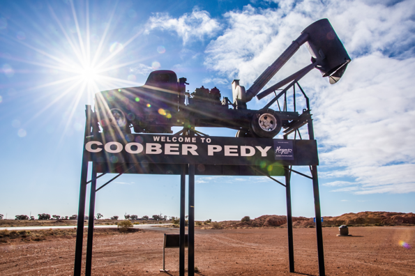
These filters are usually applied on greyscale versions of the image. So we’ll convert the image to greyscale.
test_image = test_image.convert("L") # convert to greyscale
test_image

That’s better. Let’s look at some filters.
Filters
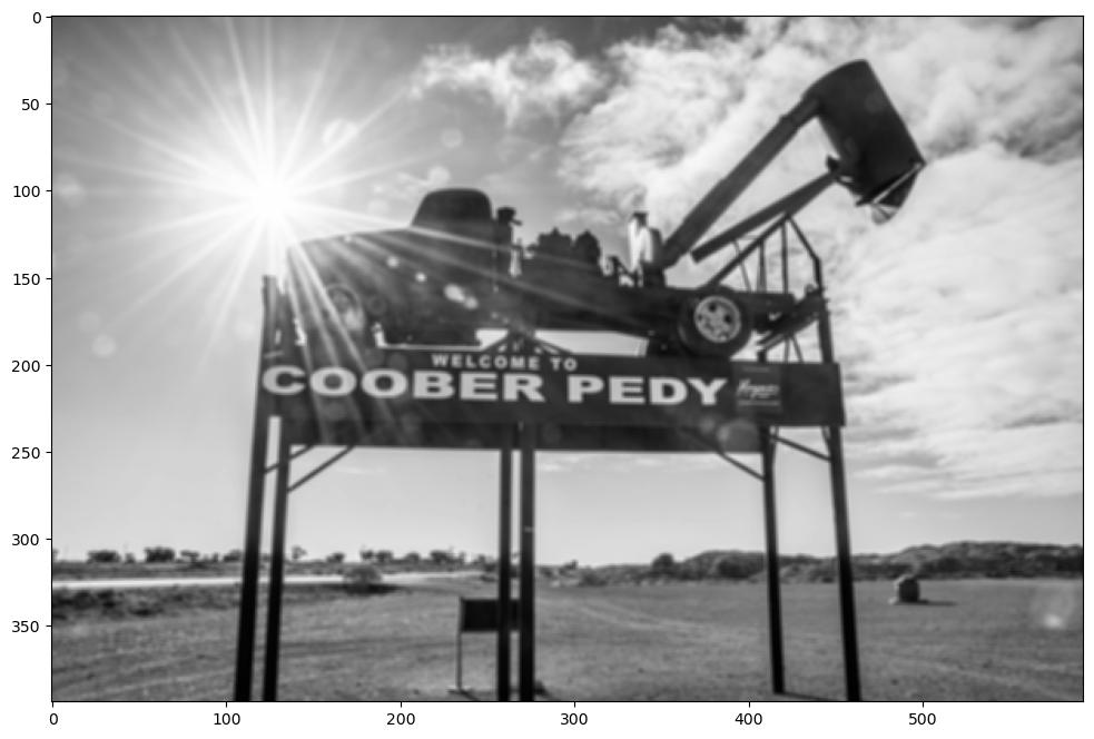
Identity
This filter leaves the image intact with no changes.
identity = np.array(([0, 0, 0], [0, 1, 0], [0, 0, 0]))
identity
array([[0, 0, 0],
       [0, 1, 0],
       [0, 0, 0]])
image_array = np.asarray(test_image)
filtered_im = convolve(image_array, identity)
fsize = (12, 8)
plt.figure(figsize=fsize)
plt.imshow(filtered_im, cmap="gray");

Random
First, let’s establish a baseline. We’ll use random numbers as our filter and see what the result is.
np.random.seed(0)
random = np.random.rand(3, 3) * 1 / 9
print(random)
[[0.06097928 0.07946549 0.06697371]
 [0.06054258 0.04707276 0.07176601]
 [0.0486208  0.09908589 0.10707364]]
Let’s make a function to view the image after it has been filtered.
def show_filtered_image(image, kernel, absv=False):
    image_array = np.asarray(image)
    filtered_im = convolve(image_array, kernel)
    plt.figure(figsize=fsize)
    if absv:
        plt.imshow(np.absolute(filtered_im), cmap="gray")
    else:
        plt.imshow(filtered_im, cmap="gray")
show_filtered_image(test_image, random)

Randomly generated filters will usually perform some sort of slightly distorted blurring. Blurring is actually a common (and sometimes desired) effect, so let’s look at that next.
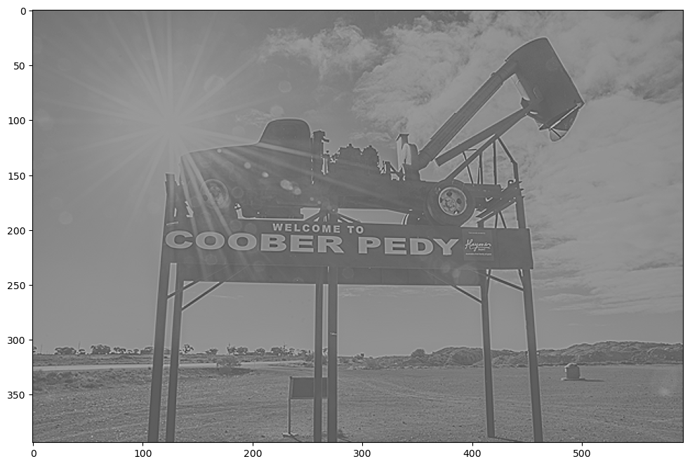
Blur
One of the things you can do with a filter is blur the entire image. To do that without creating additional distortions, we can convolve the image with a filter with the same value everywhere. We can use 1/9 to keep the magnitude the same, but the effect would be the same with any number (after normalizing).
const = 1 / 9
blur = np.array(([const, const, const], [const, const, const], [const, const, const]))
print(blur)
[[0.11111111 0.11111111 0.11111111]
 [0.11111111 0.11111111 0.11111111]
 [0.11111111 0.11111111 0.11111111]]
show_filtered_image(test_image, blur)
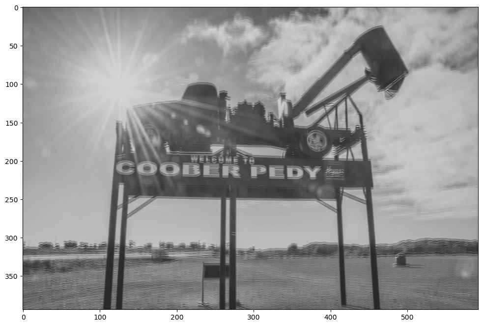
Sharpen
We can also sharpen the images with a specially designed filter.
sharpen = np.array(([0, -1, 0], [-1, 5, -1], [0, -1, 0]))
print(sharpen)
[[ 0 -1  0]
 [-1  5 -1]
 [ 0 -1  0]]
show_filtered_image(test_image, sharpen)
Why did the image become all gray? That’s because our filter had negative numbers in it, so our image values go from being [0, 255] to [-255, 255]. Matplotlib has to correct for this so it does a linear transformation of \(M_{gray} = (M_{orig} + 255) / 2\)
This takes all the 0 values in the original image, which were dark, and changes them to 125, which is gray. One way to get around this would be to square or take the absolute value of the numbers, but then we lose the sign information. For now we’d like to keep it, so we’ll leave them how they are.
Sobel
Now let’s look at Sobel filters (also known as Sobel operators). They are among the most common filters in computer vision. The Sobel operator is an approximation of the derivative of an image and is used to find lines in an image.
For most of the operators we’ll look at, there are actually four different varieties:
- Positive vertical
- Negative vertical
- Positive horizontal
- Negative horizontal
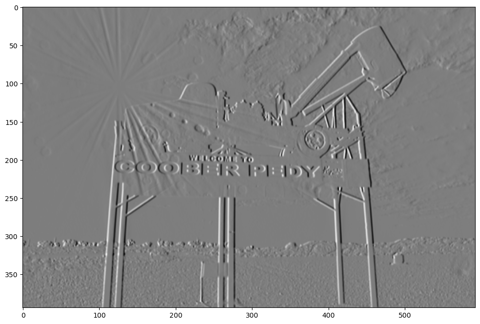
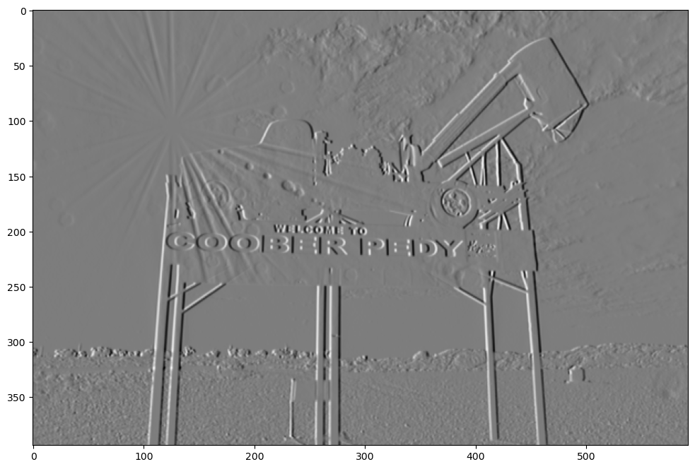
Let’s start by looking at the positive vertical one.
sobel_vert = np.array(([1, 0, -1], [2, 0, -2], [1, 0, -1]))
print(sobel_vert)
[[ 1  0 -1]
 [ 2  0 -2]
 [ 1  0 -1]]
show_filtered_image(test_image, sobel_vert)
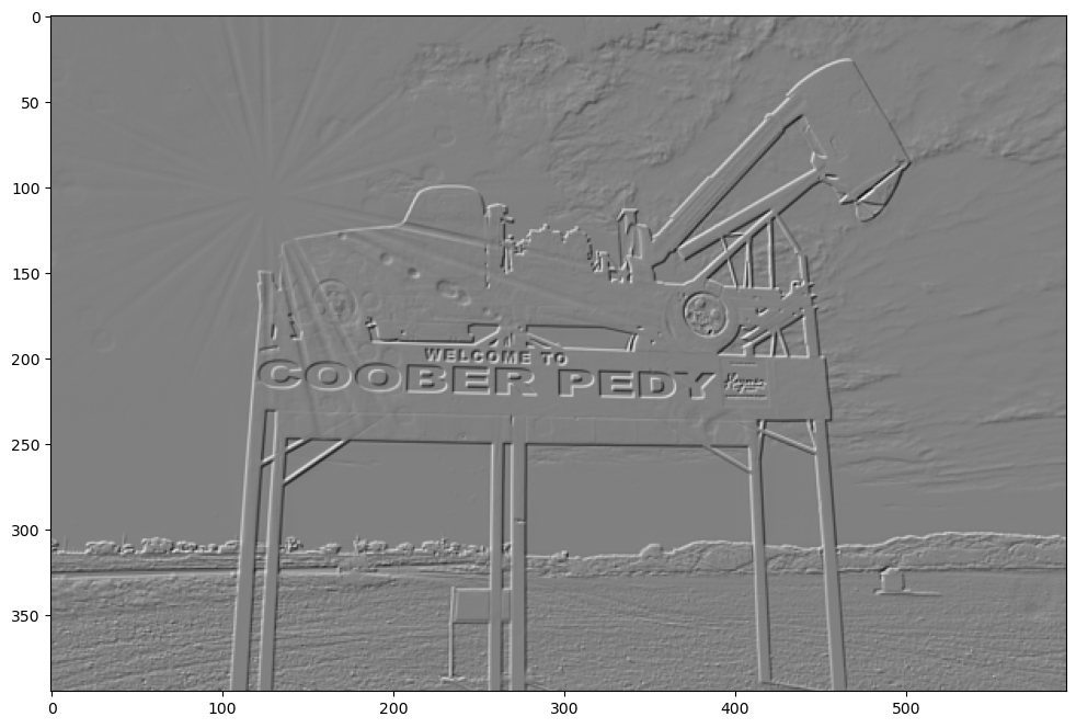
Now let’s look at the negative vertical filter.
sobel_vert_neg = np.array(([-1, 0, 1], [-2, 0, 2], [-1, 0, 1]))
print(sobel_vert_neg)
[[-1  0  1]
 [-2  0  2]
 [-1  0  1]]
show_filtered_image(test_image, sobel_vert_neg)
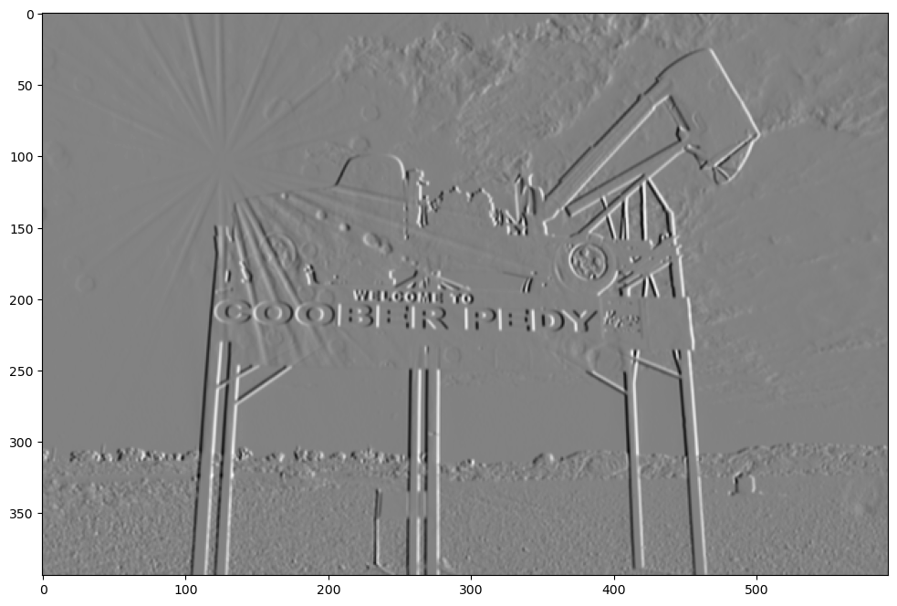
As you can see, the resulting image is very similar, and both of them do a good job at highlighting the vertical lines. But there’s a key difference in there. Can you see it? The positive filter has made the left sides of the vertical lines high values and the right side low values. The high values are whiter and the low values are blacker, so the positive vertical filter has highlighted all the vertical lines by making the left side more white and the right side more dark. Now take a look at the negative filter. In that image, the left sides of the vertical lines are dark and the right sides are light.
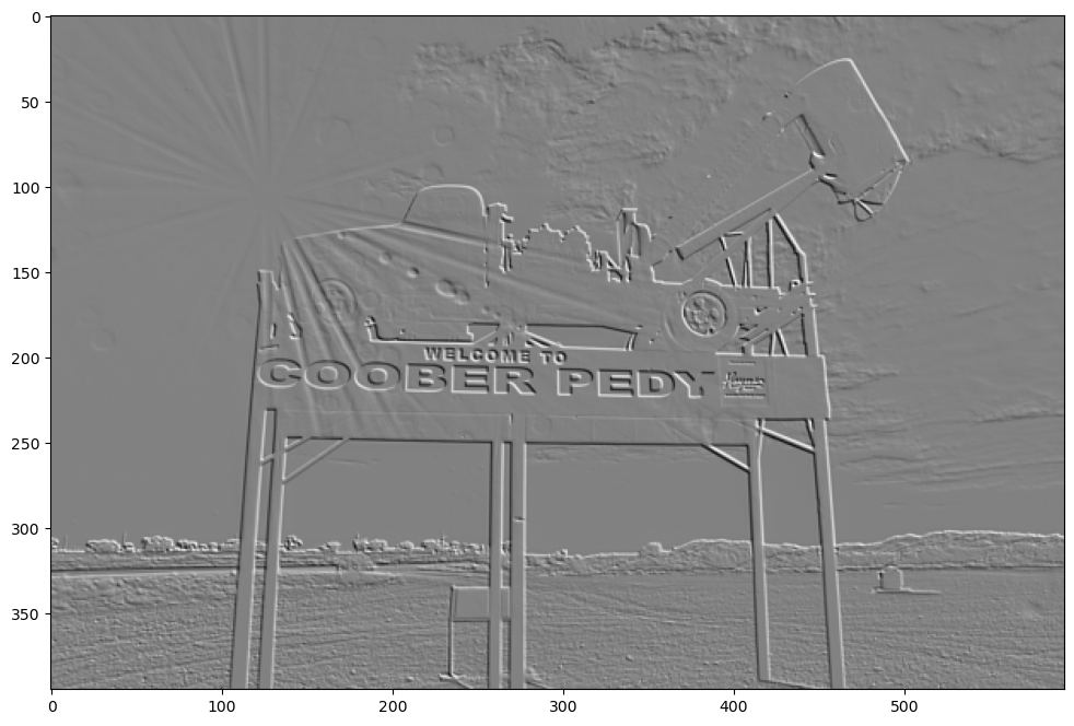
Now let’s look at the horizontal Sobel Filter and compare that.
sobel_hor = np.array(([1, 2, 1], [0, 0, 0], [-1, -2, -1]))
print(sobel_hor)
[[ 1  2  1]
 [ 0  0  0]
 [-1 -2 -1]]
show_filtered_image(test_image, sobel_hor)
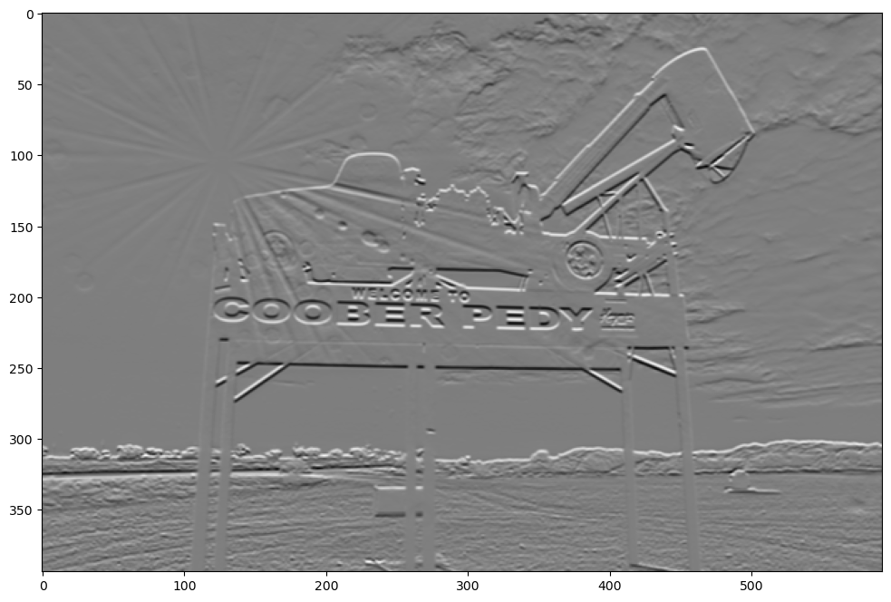
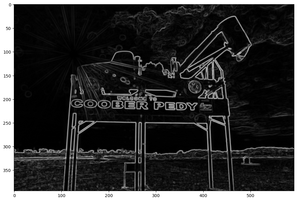
Notice that the horizontal lines are much more emphasized with the horizontal Sobel filter. The negative version does the same thing except flips the light and dark sides of the horizontal line. Filters can be combined in interesting ways to create new filters. For example, combining a Sobel vertical with a horizontal Sobel filter make a great edge detection filter.
image_array = np.asarray(test_image.convert("L"))
sobel_vert_im = convolve(image_array, sobel_vert)
sobel_hor_im = convolve(image_array, sobel_hor)
sobel_edge_detector = np.sqrt(sobel_hor_im**2 + sobel_vert_im**2)
plt.figure(figsize=fsize)
plt.imshow(sobel_edge_detector, cmap="gray");
Gaussian blur
gaussian_blur = (1 / 16) * np.array(([1, 2, 1], [2, 4, 2], [1, 2, 1]))
gaussian_blur
array([[0.0625, 0.125 , 0.0625],
       [0.125 , 0.25  , 0.125 ],
       [0.0625, 0.125 , 0.0625]])
show_filtered_image(test_image, gaussian_blur)

Gaussian blur filters are often used before a Sobel edge detection to remove some of the high frequency artifacts that appear like edges to the operator. Let’s take a look.
blurred_im = convolve(image_array, gaussian_blur)
sobel_vert_im_blurred = convolve(blurred_im, sobel_vert)
sobel_hor_im_blurred = convolve(blurred_im, sobel_hor)
sobel_edge_detector_blurred = np.sqrt(sobel_hor_im_blurred**2 + sobel_vert_im_blurred**2)
plt.figure(figsize=fsize)
plt.imshow(sobel_edge_detector_blurred, cmap="gray");

Sobel Feldman
The Sobel operator is also called the Sobel-Feldman operator (they worked together at Stanford Artificial Intelligence Laboratory (SAIL)). They also produced a slightly refined filter, which is also called a Sobel-Feldman operator. It’s similar to the vertical line detector above but the ratios are slightly different.
sobel_feldman = np.array(([3, 0, -3], [10, 0, -10], [3, 0, -3]))
print(sobel_feldman)
[[  3   0  -3]
 [ 10   0 -10]
 [  3   0  -3]]
show_filtered_image(test_image, sobel_feldman)

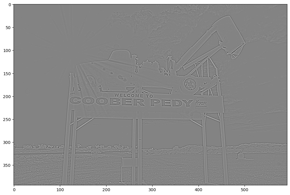
Scharr
Another famous filter is the Scharr filter. Again, it’s got a very similar look to the Sobel filter but the ratio is different.
scharr_filter = np.array(([47, 0, -47], [162, 0, -162], [47, 0, -47]))
print(scharr_filter)
[[  47    0  -47]
 [ 162    0 -162]
 [  47    0  -47]]
show_filtered_image(test_image, scharr_filter)
Robert’s Cross
Another pair of filters are known as Robert’s Cross.
roberts_cross_x = np.array(([1, 0], [0, -1]))
print(roberts_cross_x)
[[ 1  0]
 [ 0 -1]]
show_filtered_image(test_image, roberts_cross_x)
roberts_cross_y = np.array(([0, 1], [-1, 0]))
show_filtered_image(test_image, roberts_cross_y)
LaPlace
This filter is especially good at edge detection
pos_laplace = np.array(([0, 1, 0], [1, -4, 1], [0, 1, 0]))
pos_laplace
array([[ 0,  1,  0],
       [ 1, -4,  1],
       [ 0,  1,  0]])
show_filtered_image(test_image, pos_laplace)
Prewitt
prewitt = np.array(([1, 0, -1], [1, 0, -1], [1, 0, -1]))
prewitt
array([[ 1,  0, -1],
       [ 1,  0, -1],
       [ 1,  0, -1]])
show_filtered_image(test_image, prewitt)

Double
There are lots of effects that be found. Just from playing around I found this one that makes it look like the image is doubled.
double = np.array(([1,10,1], [-1,-10,-1], [1,10,1]))
show_filtered_image(test_image, double)