
Distributions are super important. In this post, I’ll talk about some common distributions, how to plot them, and what they can be used for.
Table of Contents
Distributions can be categorized as discrete or continuous based on whether the variable is discrete or continuous.
import math

import matplotlib.pyplot as plt
import numpy as np
import seaborn as sns
from scipy.stats import binom, norm, pareto, poisson
from tweedie import tweedie # used for tweedie distribution; download with `pip install tweedie`
# set seed
np.random.seed(0)
Continuous Distributions
Continuous Uniform Distribution
The most basic distribution is the uniform distribution. In this case every value between the limits is equally likely to be called. These can be continuous or discrete. Continuous uniform distributions are also called rectangular distributions.
Plot
def plot_hist(bins):
    num_bins = len(bins) - 1
    plt.xlabel('Variable')
    plt.ylabel('Count')
    plt.title(f"Continuous Uniform Distribution with {num_bins} Bins")
    plt.show()
num_samples = 10000
x = np.random.uniform(0, 1, num_samples)
num_bins = 20
count, bins, ignored = plt.hist(x, bins=num_bins, color='g', alpha=0.9)
plot_hist(bins)
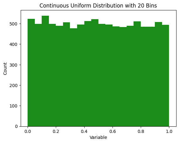
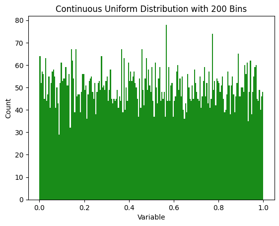
Note that the number of bins used to plot it can make it look more or less spiky. Here’s the same data plotted with 200 bins.
num_bins = 200
count, bins, ignored = plt.hist(x, bins=num_bins, color='g', alpha=0.9)
plot_hist(bins)
Uses
Whether things are truly continuously distributed or not can be a bit of a question of definition. If time and space are quantized, then nothing in the physical world is truly a continuous uniform distribution. But these things are close enough. Some uniform distributions are:
- Random number generators (in the ideal case)
- If you show up to a bus stop where the bus arrives every hour but you don’t know when, the arrival time will be a continuous distribution from 0-60 minutes
- Timing of asteroid impacts (roughly - it would only be continuous given a steady state of the universe, so doesn’t work for very long time scales)
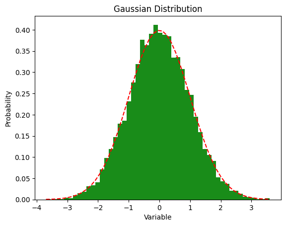
Gaussian (or Normal) Distribution
Gaussian distributions are all around us. These are the famous bell curves. I’ve found that physicists are more likely to say “Gaussian” and mathematicians are more likely to say “normal”. It seems that “normal” is more popular, although old habits die hard, so I still say “Gaussian”.
Equation
\[f(x) = \frac{e^{-\frac{x^2}{2}}}{\sqrt{2\pi} }\]Or, with more parameters:
\[f(x) = \frac{1}{\sigma \sqrt{2\pi} } e^{-\frac{1}{2}\left(\frac{x-\mu}{\sigma}\right)^2}\]Many distributions look roughly Gaussian but are not truly Gaussian. A paper on “The unicorn, the normal curve, and other improbable creatures” looked at 440 real datasets and found that none of them were perfectly normally distributed.
Plot
fig = plt.figure()

mean = 0
standard_deviation = 1
x = np.random.normal(loc=mean, scale=standard_deviation, size=num_samples)

num_bins = 50
n, bins, patches = plt.hist(x, num_bins, density=True, color='g', alpha=0.9)

# add a line
y = norm.pdf(bins, loc=mean, scale=standard_deviation)
plt.plot(bins, y, 'r--')

plt.xlabel('Variable')
plt.ylabel('Probability')

plt.title("Gaussian Distribution")
plt.show()
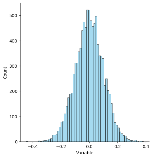
You can also do this with seaborn and displot.
mu, sigma = 0, 0.1 # mean and standard deviation
s = np.random.normal(mu, sigma, num_samples)
ax = sns.displot(s, color='skyblue')
ax.set(xlabel='Variable', ylabel='Count');
Uses
- Height is a famous example of a Gaussian distribution
- Test scores on standardized tests are roughly Gaussian
- Blood pressure of healthy populations
- Birth weight
Discrete Distributions
Lots of distributions aren’t continuous, they deal with discrete predictions. For example, you can’t flip 7.5 heads after 15 tries.
Discrete Uniform Distribution
Lots of things are discrete uniform distribution.
Plot
x = np.random.randint(0, 10, num_samples)
count, bins, ignored = plt.hist(x, color='g', alpha=0.9, rwidth=0.9)
num_bins = len(bins) - 1
plt.xlabel('Variable')
plt.ylabel('Count')
plt.title(f"Discrete Uniform Distribution")
plt.show()
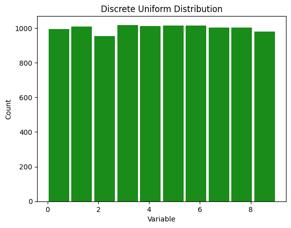
Uses
- The results of rolling a die
- The card number from a card randomly drawn from a deck
- Winning lottery numbers
- Birthdays aren’t perfectly uniform because they tend to cluster for a variety of reasons, but they are close to uniform
Bernoulli Distribution
The Bernoulli distribution is one of the simplest discrete probability distributions, serving as the basis for understanding more complex distributions like the binomial distribution. It represents the outcome of a single experiment which can result in just two outcomes: success or failure. The Bernoulli distribution is the discrete probability distribution of a random variable which takes the value 1 with probability p and the value 0 with probability q=1−p.
Plot
Consider an experiment with a single trial, like a medical test, where the probability of getting a positive (success) is 10%. To simulate this, we can do:
prob_success = 0.1
x = np.random.binomial(n=1, p=prob_success)
print(f"In this experiment, we got heads {x} times")
In this experiment, we got heads 0 times
This will output either 0 (no heads) or 1 (heads). To see the distribution of a large number of such experiments, we run multiple trials.
num_samples = 1000
data = np.random.binomial(n=1, p=prob_success, size=num_samples)

# Count occurrences of 0 and 1
successes = np.count_nonzero(data == 1)
failures = num_samples - successes

# Plotting
fig = plt.figure()
categories = ['Success', 'Failure']
counts = [successes, failures]

plt.bar(categories, counts, color='blue', alpha=0.7)
plt.xlabel('Outcome')
plt.ylabel('Count')
plt.title('Bernoulli Distribution')
plt.show()
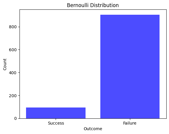
Uses
The Bernoulli distribution is used in scenarios involving a single event with two possible outcomes. Examples include:
- Flipping a coin (heads or tails).
- Success or failure of a quality check.
- In essence, any situation where there is a single trial with a “yes” or “no” type outcome can be modeled using the Bernoulli distribution.
Binomial Distribution
A binomial distribution is a discrete probability distribution that models the number of successes in a fixed number of independent trials, each with the same probability of success. It is characterized by two parameters: n, the number of trials, and p, the probability of success in each trial. It can be considered an extension of the Bernoulli distribution we saw above to multiple trials. It’s sort of like the discrete version of a Gaussian distribution.
Plot
Let’s say with run something with 100 trials, each of which has a 10% chance of happening. To run that experiment, we can do:
num_trials = 100
prob_success = 0.1
x = np.random.binomial(n=num_trials, p=prob_success)
print(f"In this experiment, we got heads {x} times")
In this experiment, we got heads 14 times
But we can run this whole experiment over and over again and see what we get.
fig = plt.figure()

# Generate data
x = np.random.binomial(n=num_trials, p=prob_success, size=num_samples)
# you could also do this with scipy like so:
# x = binom.rvs(n=num_trials, p=prob_success, size=num_samples)

num_bins = 25
# Define bin edges explicitly to avoid gaps
bin_edges = np.arange(min(x), max(x) + 2)

# Plot the histogram
plt.hist(x, bins=bin_edges, density=True, color='g', alpha=0.9, rwidth=0.9)

plt.xlabel('Variable')
plt.ylabel('Probability')

plt.title("Binomial Distribution (Bin size {})".format(num_bins))
plt.show()
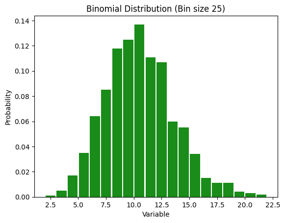
Uses
- Flipping a coin
- Shooting free throws
- Lots of things that seem to be Gaussian but are discrete
Poisson Distribution
Many real-life things follow a Poisson distribution. Poisson distributions are like binomial distributions in that they count discrete events. But it’s different in that there is no fixed number of experiments to run. Imagine a soccer game. So it’s discrete occurrences (yes/no for a goal being scored) along a continuous distribution (time).
At any moment, a goal could be scored. Thus it is continuous. There’s no specific number of “goal attempts” in a Poisson distribution.
If you wanted to find the number of shots on goal and see how many of them were goals, then it would become binomial. But if you look at it over time it’s Poisson. It’s like the limit of a binomial distribution where you have infinite attempts and each has an infinitesimal chance of being positive.
Note that Poisson and binomial distributions can’t be negative.
Equation
Mathematically, this looks like: \(P(x = k) = e^{-\lambda}\frac{\lambda^k}{k!}\)
Plot
data_poisson = poisson.rvs(mu=3, size=num_samples)
ax = sns.displot(data_poisson, color='skyblue')
ax.set(xlabel='Variable', ylabel='Count');
ax.fig.suptitle('Poisson Distribution')
Text(0.5, 0.98, 'Poisson Distribution')
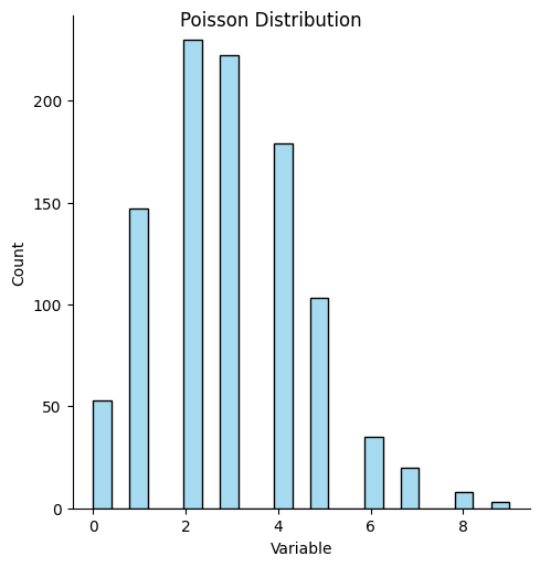
Uses
- Decay events from radioactive sources
- Meteorites hitting the Earth
- Emails sent in a day
Example
Poisson distributions are very useful in predicting rare events. If once-in-a-lifetime floods occur once every hundred years, what is the chance that we have five within a hundred-year period?
In this case \(\lambda = 1\) and \(k = 5\)
math.exp(-1)*(1**5/math.factorial(5))
0.0030656620097620196
Mixed Discrete and Continuous Distributions
Tweedie Distribution
The Tweedie distribution is a family of probability distributions that encompasses a range of other well-known distributions. It is characterized by its ability to model data that exhibit a combination of discrete and continuous features, particularly useful for datasets with a significant number of zero values but also positive continuous outcomes. This makes the Tweedie distribution ideal for applications in fields such as insurance claim modeling, financial data analysis, and ecological studies, where the distribution of observed data cannot be adequately captured by simpler, more conventional distributions.
Plot
num_params = 20
# Generate random exogenous variables, num_samples x (num_params - 1)
exog = np.random.rand(num_samples, num_params - 1)

# Add a column of ones to the exogenous variables, num_samples x num_params
exog = np.hstack((np.ones((num_samples, 1)), exog))

# Generate random coefficients for the exogenous variables, num_params x 1
beta = np.concatenate(([500], np.random.randint(-100, 100, num_params - 1))) / 100

# Compute the linear predictor, num_samples x 1
eta = np.dot(exog, beta)

# Compute the mean of the Tweedie distribution, num_samples x 1
mu = np.exp(eta)

# Generate random samples from the Tweedie distribution, num_samples x 1
x = tweedie(mu=mu, p=1.5, phi=20).rvs(num_samples)
num_bins = 50
n, bins, patches = plt.hist(x, num_bins, density=True, color='g', alpha=0.9, rwidth=0.9)
plt.xlabel('Variable')
plt.ylabel('Probability')

plt.title("Tweedie Distribution")
plt.show()
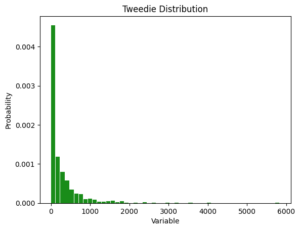
Uses
Tweedie distributions are most common when values are a combination of zero values and some continuous values, such as the following:
- Insurance claims
- Number of each type of various species in an area
- Healthcare expenditures
Power Law Distribution
Power law distributions are pervasive in our world. These distributions describe phenomena where small occurrences are extremely common, while large occurrences are extremely rare. Unlike Gaussian distributions, power law distributions do not centralize around a mean value; instead, they are characterized by a long tail, where a few large values dominate.
Equation
The general form of a power law distribution is given by:
\[P(x) = Cx^{-\alpha}\]where
- P(x) is the probability of observing the event of size x
- C is a normalization constant ensuring the probabilities sum up to 1
- α is a positive constant that determines the distribution’s shape.
Pareto and Zipf’s Distributions
The Pareto and Zipf’s (pronounced “zif’s”) distributions are instances of power laws. Pareto distributions are more common with continuous data and Zipf’s distributions are more common with discrete data. They’re both very important so let’s look at them separately.
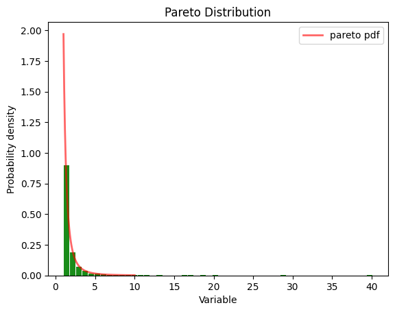
Pareto Distribution - Continuous
The Pareto distribution is a specific instance of a power law distribution. It was developed by Italian economist Vilfredo Pareto to model wealth and income. This distribution encapsulates the Pareto principle or the “80/20 rule,” which suggests that 80% of the wealth is owned by 20% of the population. The Pareto distribution is seen all the time, from social issues to scientific ones.
Plot
# Distribution parameters
a = 2.0 # shape parameter
b = 1.0 # scale parameter

# Generate random samples from the distribution
pareto_samples = pareto.rvs(a, scale=b, size=1000)

# Plot the histogram of the samples
plt.hist(pareto_samples, bins=50, density=True, color='g', alpha=0.9, rwidth=0.9)

# Plot the probability density function (PDF)
x = np.linspace(pareto.ppf(0.01, a, scale=b), pareto.ppf(0.99, a, scale=b), 100)
plt.plot(x, pareto.pdf(x, a, scale=b), 'r-', lw=2, alpha=0.6, label='pareto pdf')

plt.xlabel('Variable')
plt.ylabel('Probability density')
plt.title('Pareto Distribution')
plt.legend()
plt.show()
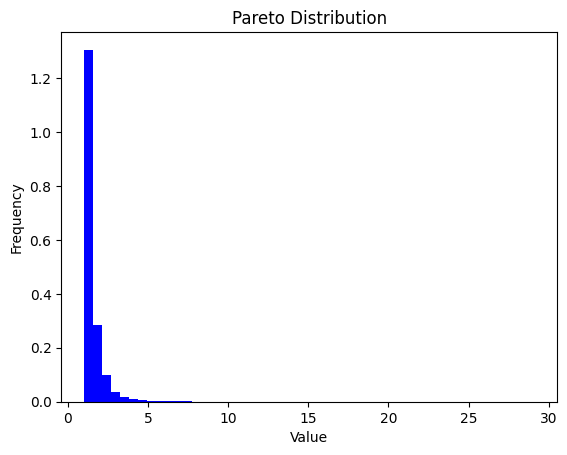
You can also generate them with numpy.
b = 3.0 # Shape parameter
samples = 10000
pareto_samples = (np.random.pareto(b, samples) + 1)
Note that the x values in the pareto distribution are continuous.
pareto_samples
array([1.67027215, 1.01475779, 2.95279024, ..., 1.58598305, 1.03600555,
       1.55869634])
plt.hist(pareto_samples, bins=50, density=True, color='blue')
plt.xlabel('Value')
plt.ylabel('Frequency')
plt.title('Pareto Distribution')
plt.show()
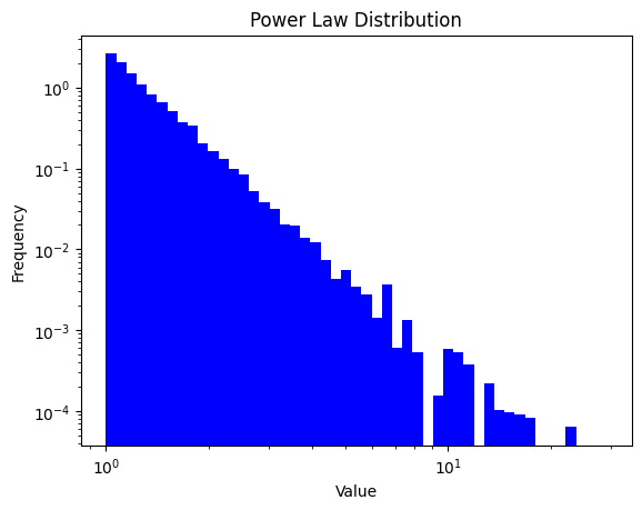
The linear plot is hard to see, so it’s common to plot it on a log scale.
plt.hist(pareto_samples, bins=np.logspace(np.log10(min(pareto_samples)), np.log10(max(pareto_samples)), 50), density=True, color='blue')
plt.gca().set_xscale("log")
plt.gca().set_yscale("log")
plt.xlabel('Value')
plt.ylabel('Frequency')
plt.title('Power Law Distribution')
plt.show()
findfont: Font family ['cmsy10'] not found. Falling back to DejaVu Sans.
findfont: Font family ['cmr10'] not found. Falling back to DejaVu Sans.
findfont: Font family ['cmtt10'] not found. Falling back to DejaVu Sans.
findfont: Font family ['cmmi10'] not found. Falling back to DejaVu Sans.
findfont: Font family ['cmb10'] not found. Falling back to DejaVu Sans.
findfont: Font family ['cmss10'] not found. Falling back to DejaVu Sans.
findfont: Font family ['cmex10'] not found. Falling back to DejaVu Sans.
Uses
- 80-20 rule
- Income and Wealth Distribution
Recursive Nature
The 80-20 rule is recursive. That is, if 20% of the people do 80% of the work, you can zoom in on those 20% and find that 20% of those do 80% of that work. So you can say something like
\((0.2)^x\) of the people do \((0.8)^x\) of the work for any \(x\).
For \(x=2\), this would be:
print(f"{(0.2)**2: .4} of the people do{(0.8)**2: .4} of the work.")
0.04 of the people do 0.64 of the work.
For \(x=3\), this would be:
print(f"{(0.2)**3: .4} of the people do{(0.8)**3: .4} of the work.")
0.008 of the people do 0.512 of the work.
Zipf’s Distribution - Discrete
The Zipf distribution, or Zipf’s law, is another flavor of power law distributions, named after the American linguist George Zipf. It specifically describes the phenomenon where the frequency of an item is inversely proportional to its rank in a frequency table. Commonly observed in linguistics, where the most frequent word occurs twice as often as the second most frequent word, thrice as often as the third most frequent word, and so on (see this Vsauce video for more). Unlike the Pareto distribution, which primarily models the upper tail of distributions, Zipf’s law applies more broadly, capturing the essence of rank-size distributions.
Plot
alpha = 2.5
size = 1000  # Number of samples
zipf_samples = np.random.zipf(alpha, size)

# Plotting the histogram
plt.hist(zipf_samples, bins=np.linspace(1, 50, 50), density=True, alpha=0.75, color='blue')
plt.title('Zipf (Power Law) Distribution')
plt.xlabel('Value')
plt.ylabel('Frequency')
plt.yscale('log')
plt.show()
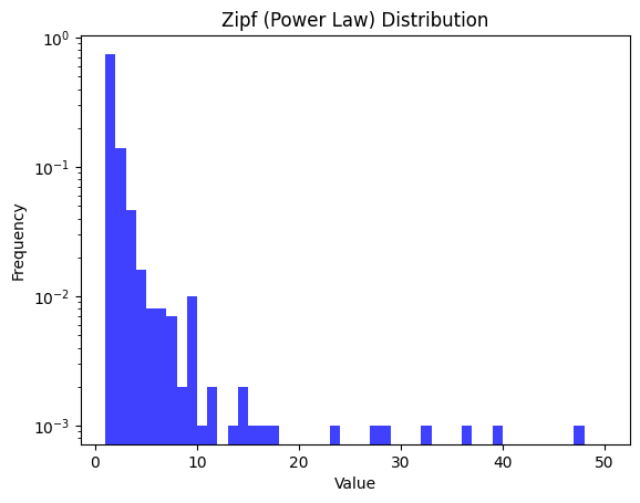
Note that now the values are discrete.
zipf_samples[:10]
array([1, 1, 1, 5, 1, 3, 1, 1, 1, 3])
Uses
- Linguistics (word usage)
- Internet traffic (number of visitors to websites)
- File size in a computer
- Earthquakes